Matcher: Flexible Optics Matching in Ocelot

note

The new Matcher will be available from version 26.03 and is currently in the dev branch.

ocelot.cpbd.matcher is a new object-oriented matching API. It is designed to be more flexible and clearer than the legacy cpbd.match.py workflow, while staying physics-oriented.

Why a New Matcher?

Compared with legacy match.py, matcher gives you:

• A clear object model: MatchProblem + variables + targets + objectives.
• Generic variable control: vary_element(...) can vary any numeric quantity (element field) of any element (for example k1, angle, l, cavity v, cavity phi).
• Per-variable bounds via limits=(low, high).
• Per-target controls: weight, tol, relation.
• Generic user-defined objective functions (minimize_function, objective_function) and custom objective classes.
• Linked variables for shared hardware (for example one power supply driving several quads).
• Direct support for Twiss targets, global Twiss limits, Twiss deltas, and R-matrix targets.
• Better diagnostics in solve result (target_reports, objective_reports).

Legacy cpbd.match.py can still coexist. New scripts can adopt matcher incrementally.

Matching Model

Think in three blocks:

1. Variables (Vary): what optimizer is allowed to change.
2. Targets (Target): constraints you want to satisfy.
3. Objectives (Objective): extra terms to minimize.

Everything contributes residuals. The solver minimizes:

sum(weighted_residual_i^2).

Main Classes and Their Roles

• MatchProblem: central container (lattice, initial Twiss, periodic mode, variables, targets, objectives, solve/evaluate entry points).
• Vary: one optimization knob.
• PowerSupplyVary: one knob applied to multiple elements with optional scales.
• Target subclasses: Twiss, Twiss delta, global Twiss, R-matrix, etc.
• Objective subclasses: generic function objective, I5 objective, custom user objectives.
• MatchState: optics snapshot for one evaluation.
• MatchResult: solve output and reports.

MatchState (what you can use in custom objectives)

During each evaluation, matcher builds a MatchState with:

• twiss_start: effective initial Twiss used in this evaluation.
• twiss_by_element: dictionary element -> Twiss.
• twiss_sequence: ordered list of Twiss along lattice sequence.
• twiss_end: Twiss at end of line for current state.
• r_matrix(start, end): cached transfer matrix accessor return.

Important for periodic matching:

• periodic=False: start Twiss is your current twiss0.
• periodic=True: matcher computes periodic Twiss from current lattice and uses it as twiss_start. In this mode, varying initial Twiss directly is usually not meaningful.

Workflow

Typical solve flow:

1. Create MatchProblem(lat, tw0, periodic=...).
2. Add variables (vary_element, vary_twiss, vary_linked_elements).
3. Add targets (target_twiss, target_global, target_twiss_delta, target_rmatrix, target_rmatrix_block, ...).
4. Add objectives (minimize_function, objective_function, minimize_i5_integral, custom objective).
5. Run solve(solver=..., max_iter=..., tol=...).
6. Inspect result.variables, result.target_reports, result.objective_reports, result.merit.

Solvers and Bounds

Pass solver in problem.solve(solver="...").

Bounds-capable solvers:

• ls_trf (least-squares trust-region reflective, recommended default)
• ls_dogbox (least-squares dogbox)
• least_squares (alias to ls_trf)
• simplex (alias for nelder-mead)
• nelder-mead
• powell
• lbfgsb (alias for l-bfgs-b)
• l-bfgs-b
• slsqp

Solvers without bounds support:

• ls_lm
• bfgs
• cg

If any active variable has finite bounds and solver does not support bounds, matcher raises ValueError (intentional hard error, not warning).

objective_function Modes

objective_function(func, mode=...) supports:

• mode="residual": function output is treated directly as residual(s).
• mode="minimize": residual is func(state) - target.
• mode="target": relation/tolerance logic (==, <=, >=, etc.).

Practical note:

• residual and minimize(target=0) are equivalent for same function output.
• Use residual when your function already returns an error-like vector.
• Use minimize for clearer intent with explicit scalar target.

Limitations and Practical Notes

• This is local nonlinear optimization. Good initial conditions still matter.
• Large one-shot problems with many knobs/constraints can converge to poor optics. Regularization and staged matching are often better.
• Weights and scales matter. Normalize residual terms so no single term dominates unintentionally.
• For periodic=True, fitting entrance Twiss via vary_twiss(...) is usually not the right control strategy.

Examples

1) Generic Pattern (I5 as regular objective)

Treat I5 like any other objective term instead of build in shortcut problem.minimize_i5_integral(weight=1e14).

import numpy as np

from ocelot.cpbd.matcher import MatchProblem
from ocelot.cpbd.beam_params import radiation_integrals

# Assume: lat, tw0, q1, q2, end are already defined
problem = MatchProblem(lat, tw0, periodic=True)

# Variables
problem.vary_element(q1, quantity="k1", limits=(-5, 5))
problem.vary_element(q2, quantity="k1", limits=(-5, 5))

# Twiss targets
problem.target_twiss(end, "beta_x", 12.0, weight=1e6)
problem.target_twiss(end, "beta_y", 9.0, weight=1e6)

# I5 as a generic objective
problem.minimize_function(
    lambda state: radiation_integrals(state.lat, state.twiss_start, nsuperperiod=1)[4],
    name="I5",
    weight=1e14,
)

# Or use built-in shortcut:
# problem.minimize_i5_integral(weight=1e14)

result = problem.solve(solver="ls_trf", max_iter=300)
print(result.success, result.merit)

2) Custom Integral Objective

You can minimize any function of MatchState.

How it works:

• You pass a callable to problem.minimize_function(...).
• Matcher stores it.
• On every evaluation/iteration, matcher builds the current MatchState internally and calls your function as func(state).
• You do not create state yourself.

Important Python note:

• In lambda state: ..., state is just the function argument name.
• It can be any name (lambda ms: ... is equivalent).
• The matcher passes the current MatchState object into that argument.

Equivalent forms:

# lambda form
problem.minimize_function(
    lambda state: np.trapz(
        [tw.beta_x for tw in state.twiss_sequence],
        [tw.s for tw in state.twiss_sequence],
    ),
    name="int_beta_x_ds",
    weight=1.0,
)

# named-function form (exact same behavior)
def integral_beta_x(match_state):
    return np.trapz(
        [tw.beta_x for tw in match_state.twiss_sequence],
        [tw.s for tw in match_state.twiss_sequence],
    )

problem.minimize_function(integral_beta_x, name="int_beta_x_ds", weight=1.0)

3) Custom Objective Class

Use custom class when you need reusable logic.

import numpy as np
from ocelot.cpbd.matcher import Objective

class EndSObjective(Objective):
    def __init__(self, target_s, **kwargs):
        super().__init__(**kwargs)
        self.target_s = float(target_s)

    def residuals(self, state):
        # Matcher minimizes sum(residual^2)
        return np.array([state.twiss_end.s - self.target_s], dtype=float)

# Add custom objective to problem
problem.add_objective(EndSObjective(target_s=12.0, name="end_s_obj", weight=1e6))

4) Global Beta Limits

# Keep beta_x and beta_y below limits everywhere
problem.target_global(
    quantity="beta_x",
    value=30.0,
    relation="<=",
    weight=1e6,
    tol=0.0,
    name="beta_x_max",
)

problem.target_global(
    quantity="beta_y",
    value=35.0,
    relation="<=",
    weight=1e6,
    tol=0.0,
    name="beta_y_max",
)

result = problem.solve(solver="ls_trf", max_iter=300)
print(result.success, result.merit)

5) Vary Initial Twiss

Use when entrance optics are unknown and must be fitted.

from ocelot.cpbd.matcher import MatchProblem

# Assume: lat, tw0, end are already defined
problem = MatchProblem(lat, tw0, periodic=False)

# Fit entrance optics
problem.vary_twiss(quantity="beta_x", limits=(0.1, 300.0), name="bx0")
problem.vary_twiss(quantity="alpha_x", limits=(-20.0, 20.0), name="ax0")

# Optional: also fit dispersion
problem.vary_twiss(quantity="Dx", limits=(-2.0, 2.0), name="Dx0")
problem.vary_twiss(quantity="Dxp", limits=(-1.0, 1.0), name="Dxp0")

# Match Twiss at end
problem.target_twiss(end, "beta_x", 12.0, weight=1e6)
problem.target_twiss(end, "alpha_x", 0.0, weight=1e6)

result = problem.solve(solver="ls_trf", max_iter=300)
print(result.success, result.variables["bx0"], result.variables["ax0"])

6) Vary Bend Angle and Drift Length

vary_element(...) is generic, not only for quadrupole k1.

from ocelot.cpbd.matcher import MatchProblem
from ocelot.cpbd.elements import Bend, Drift, Marker
from ocelot.cpbd.magnetic_lattice import MagneticLattice

# Simple line
start = Marker(eid="S")
b = Bend(l=1.0, angle=0.20, eid="B1")
d = Drift(l=3.0, eid="D1")
end = Marker(eid="E")
lat = MagneticLattice((start, b, d, end))

problem = MatchProblem(lat, tw0, periodic=False)

# Vary bend angle with bounds
problem.vary_element(b, quantity="angle", limits=(0.15, 0.30), name="B1_angle")

# Vary drift length with bounds
problem.vary_element(d, quantity="l", limits=(2.0, 5.0), name="D1_l")

# Example targets
problem.target_twiss(end, "Dx", 0.12, weight=1e6)
problem.target_twiss(end, "s", 4.2, weight=1e6)

result = problem.solve(solver="ls_trf", max_iter=200)
print(result.success, result.variables["B1_angle"], result.variables["D1_l"])

7) Vary Cavity Voltage/Phase and Target End Energy

Cavity quantities are standard element fields:

• v in GV
• phi in degrees

End energy is Twiss quantity E in GeV.

import numpy as np
from ocelot.cpbd.matcher import MatchProblem
from ocelot.cpbd.elements import Cavity, Marker
from ocelot.cpbd.magnetic_lattice import MagneticLattice

start = Marker(eid="S")
cav = Cavity(l=0.5, v=0.02, phi=0.0, freq=1.3e9, eid="C1")
end = Marker(eid="E")
lat = MagneticLattice((start, cav, end))

problem = MatchProblem(lat, tw0, periodic=False)

# Example 1: fit voltage to reach final energy
problem.vary_element(cav, quantity="v", limits=(0.0, 0.05), name="C1_v")
problem.target_twiss(end, "E", value=1.03, weight=1e6)
result = problem.solve(solver="ls_trf", max_iter=200)
print("voltage fit:", result.success, result.variables["C1_v"])

# Example 2: fit phase to reach final energy (keep v fixed)
cav.v = 0.03
cav.phi = 20.0
problem2 = MatchProblem(lat, tw0, periodic=False)
problem2.vary_element(cav, quantity="phi", limits=(0.0, 60.0), name="C1_phi")
problem2.target_twiss(end, "E", value=1.0 + 0.03 * np.cos(np.deg2rad(30.0)), weight=1e6)
result2 = problem2.solve(solver="ls_trf", max_iter=200)
print("phase fit:", result2.success, result2.variables["C1_phi"])

8) Target One R-matrix Element Between Two Elements

You can constrain any transfer matrix entry R[i, j] between two elements in lattice order (start <= end). This can be internal markers, not only line start/end.

from ocelot.cpbd.matcher import MatchProblem
from ocelot.cpbd.elements import Drift, Marker
from ocelot.cpbd.magnetic_lattice import MagneticLattice

start = Marker(eid="S")
d0 = Drift(l=0.4, eid="D0")
m1 = Marker(eid="M1")
dvar = Drift(l=1.1, eid="DVAR")
m2 = Marker(eid="M2")
d2 = Drift(l=0.7, eid="D2")
end = Marker(eid="E")
lat = MagneticLattice((start, d0, m1, dvar, m2, d2, end))

problem = MatchProblem(lat, tw0, periodic=False)
problem.vary_element(dvar, quantity="l", limits=(0.0, 5.0), name="DVAR_l")

# Match R12 (Python indices i=0, j=1) between M1 and M2
problem.target_rmatrix(m1, m2, i=0, j=1, value=2.7, weight=1e6)

result = problem.solve(solver="ls_trf", max_iter=200)
print(result.success, result.variables["DVAR_l"])

9) Two Quadrupoles on One Power Supply

One shared knob can control multiple elements.

from ocelot.cpbd.matcher import MatchProblem

# Assume: lat, tw0, q1, q2, end are already defined
problem = MatchProblem(lat, tw0, periodic=False)

# One knob drives both quadrupoles.
# Example below uses opposite polarity.
ps = problem.vary_linked_elements(
    elements=[q1, q2],
    scales=[1.0, -1.0],
    quantity="k1",
    name="PS_Q1Q2",
    limits=(-2.0, 2.0),
)

problem.target_twiss(end, "beta_x", 12.0, weight=1e6)
problem.target_twiss(end, "beta_y", 9.0, weight=1e6)

result = problem.solve(solver="ls_trf", max_iter=300)
print(result.success, result.variables["PS_Q1Q2"])
print("q1.k1 =", q1.k1, "q2.k1 =", q2.k1)

10) Regularization (Small and Smooth Quad Strengths)

Regularization is straightforward with residual-vector objectives.

import numpy as np

# Assume quads are ordered along s:
quads = [q1, q2, q3, q4, q5]

# Optional reference profile (here: all zeros)
k_ref = np.zeros(len(quads))

# Normalization scales to control relative strength of penalties
k_scale = 0.2     # absolute strength penalty
dk_scale = 0.05   # neighbor-difference penalty

# Penalize large strengths: sum((k_i - k_ref_i)^2)
problem.objective_function(
    lambda state: (np.array([q.k1 for q in quads]) - k_ref) / k_scale,
    mode="residual",
    name="reg_k_l2",
    weight=1.0,
)

# Penalize rapid changes: sum((k_{i+1} - k_i)^2)
problem.objective_function(
    lambda state: np.diff(np.array([q.k1 for q in quads])) / dk_scale,
    mode="residual",
    name="reg_k_smooth",
    weight=1.0,
)

11) Phase Delta Target with wrap_phase=True

For mux/muy delta targets, phase values differing by 2*pi are physically equivalent.

import numpy as np

problem.target_twiss_delta(
    start=elem1,
    end=elem2,
    quantity="mux",
    value=3.0 * np.pi / 2.0,
    relation="==",
    wrap_phase=True,  # wrap residual to [-pi, pi]
    weight=1e6,
    tol=1e-4,
    name="dmu_x_elem1_elem2",
)

Why it matters:

• Without wrapping, equivalent phases can look numerically far apart (for example -pi/2 vs 3*pi/2 gives raw -2*pi difference).
• With wrap_phase=True, residual is near zero for equivalent phase targets.

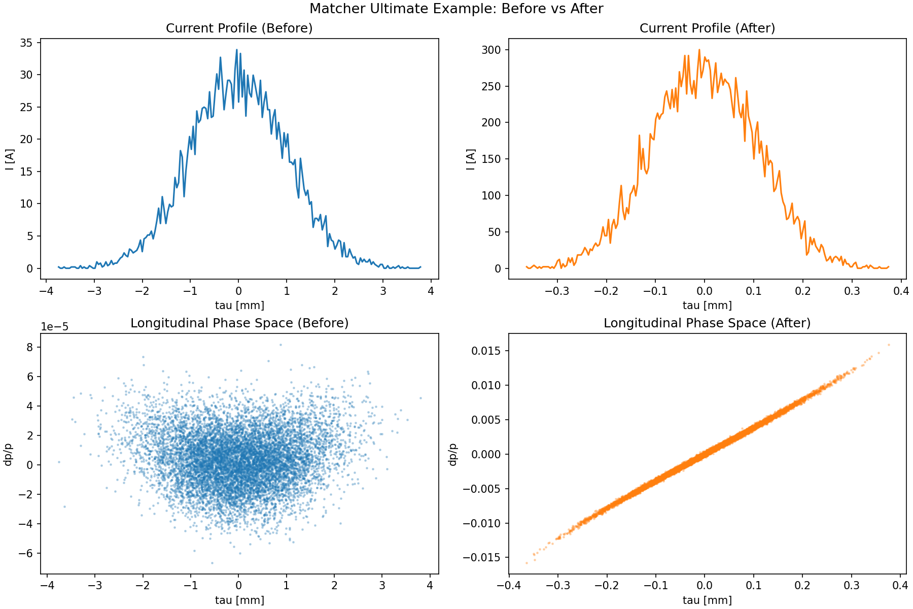
12) Ultimate Example: Custom Chicane Knob + Tracking Objective + Energy Target

Reference script:

• demos/ebeam/matcher_ex.py

This example combines three patterns in one workflow:

• Custom variable (Vary) with coupled lattice updates: one knob CHICANE_theta updates four dipole angles, edge angles (e1, e2), and chicane shoulder drifts consistently.
• Custom objective (Objective) with particle tracking inside residual evaluation: match a target peak current from tracked ParticleArray.
• Standard matcher target: final energy constraint with problem.target_twiss(end, "E", ...).

# Build a C-shape chicane section.
z_distance = 1.0
d_ref = Drift(l=0.5)
d12 = Drift(l=shoulders_from_theta(THETA0, z_distance))
d34 = Drift(l=shoulders_from_theta(THETA0, z_distance))

b1 = SBend(l=0.2, angle=-THETA0, e1=0.0, e2=-THETA0, tilt=0.0, fint=0.0, eid="B1")
b2 = SBend(l=0.2, angle=+THETA0, e1=THETA0, e2=0.0, tilt=0.0, fint=0.0, eid="B2")
b3 = SBend(l=0.2, angle=+THETA0, e1=0.0, e2=THETA0, tilt=0.0, fint=0.0, eid="B3")
b4 = SBend(l=0.2, angle=-THETA0, e1=-THETA0, e2=0.0, tilt=0.0, fint=0.0, eid="B4")
chicane = (b1, d12, b2, d_ref, b3, d34, b4)

# RF section and end marker.
c11 = Cavity(l=0.5, v=0.15, phi=0.0, freq=1.3e9, eid="C11")
c13 = Cavity(l=0.5, v=0.0166, phi=180.0, freq=3.9e9, eid="C13")
end = Marker(eid="END")

cell = [d_ref, c11, d_ref, c13, d_ref, *chicane, d_ref, end]
lat = MagneticLattice(cell)

tw0 = Twiss(beta_x=10.0, beta_y=10.0, emit_xn=1e-6, emit_yn=1e-6, E=0.005)
parray_init = generate_parray(tws=tw0, nparticles=10000, charge=250e-12,  chirp=0.0, sigma_p=SIGMA_P, sigma_tau=SIGMA_TAU_M)

# Track once before matching as a reference.
_tb, tracked_before = track(lat, copy.deepcopy(parray_init), print_progress=False)
i_before = peak_current(tracked_before)

# Create matcher problem.
problem = MatchProblem(lat, tw0)

# Custom composite variable: one theta knob drives the full chicane geometry.
def get_theta() -> float:
    return float(b2.angle)

def set_theta(theta: float) -> None:
    # 1) Update linked dipole angles.
    b1.angle = -theta
    b2.angle = +theta
    b3.angle = +theta
    b4.angle = -theta

    # 2) Update linked edge angles.
    b1.e1, b1.e2 = 0.0, -theta
    b2.e1, b2.e2 = +theta, 0.0
    b3.e1, b3.e2 = 0.0, +theta
    b4.e1, b4.e2 = -theta, 0.0

    # 3) Recompute chicane shoulder drifts from geometry.
    l_shoulder = shoulders_from_theta(theta, z_distance)
    d12.l = l_shoulder
    d34.l = l_shoulder

problem.add_variable(
    Vary(
        name="CHICANE_theta",
        getter=get_theta,
        setter=set_theta,
        limits=THETA_LIMITS,
    )
)

# Standard RF variables.
problem.vary_element(c11, quantity="v", limits=(0.10, 0.20), name="C11_v")
problem.vary_element(c11, quantity="phi", limits=(-40.0, 40.0), name="C11_phi")
problem.vary_element(c13, quantity="v", limits=(0.01, 0.025), name="C13_v")
problem.vary_element(c13, quantity="phi", limits=(90.0, 270.0), name="C13_phi")

# Custom tracking objective: peak current target.
class PeakCurrentObjective(Objective):
    """Tracking-based objective for peak current matching."""

    def __init__(self, parray_template, target_current: float, num_bins: int = 200, **kwargs):
        super().__init__(**kwargs)
        self.parray_template = parray_template
        self.target_current = float(target_current)
        self.num_bins = int(num_bins)

    def residuals(self, state):
        # Track a fresh copy each evaluation so residuals always use the same
        # initial particle distribution.
        parray = copy.deepcopy(self.parray_template)
        _tws_track, tracked = track(state.lat, parray, print_progress=False)
        i_peak = peak_current(tracked, num_bins=self.num_bins)
        return np.array([(i_peak - self.target_current) / self.target_current], dtype=float)

# Add custom objective to the problem.
problem.add_objective(
    PeakCurrentObjective(
        parray_template=parray_init,
        target_current=300,  # A
        name="peak_current_obj",
        weight=1e1,
    )
)

# Standard physics constraint: final energy at end marker (130 MeV).
problem.target_twiss(end, "E", value=0.13, weight=1e6)

# Solve.
result = problem.solve(solver="ls_trf", max_iter=MAX_ITER)

Run the full demo script:

python demos/ebeam/matcher_ex.py

Script output:

• console summary with optimized variables and achieved peak current
• generated figure: demos/ebeam/matcher_ex_before_after.png

Before/after image from the demo:

Regression + Benchmark Test

The test module unit_tests/ebeam_test/matcher/matcher_test.py includes:

• functional regression tests for matcher capabilities
• large-lattice optics cases
• benchmark timing test

Run full matcher tests:

pytest -q unit_tests/ebeam_test/matcher/matcher_test.py

Update benchmark baseline:

MATCHER_BENCH_UPDATE=1 pytest -q unit_tests/ebeam_test/matcher/matcher_test.py::test_match_optics_benchmark

Enforce speed regression guard (for example max 25% slowdown):

MATCHER_BENCH_ENFORCE=1 MATCHER_BENCH_MAX_SLOWDOWN=1.25 pytest -q unit_tests/ebeam_test/matcher/matcher_test.py::test_match_optics_benchmark