Matcher: Flexible Optics Matching in Ocelot

note

The new Matcher will be available from version 26.03 and is currently in the dev branch.

ocelot.cpbd.matcher is a new object-oriented matching API. It is designed to be more flexible and clearer than the legacy cpbd.match.py workflow, while staying physics-oriented.

Why a New Matcher?

Compared with legacy match.py, matcher gives you:

• A clear object model: MatchProblem + variables + targets + objectives.
• Generic variable control: vary_element(...) can vary any numeric quantity (element field) of any element (for example k1, angle, l, cavity v, cavity phi).
• Per-variable bounds via limits=(low, high).
• Per-target controls: weight, tol, relation.
• Generic user-defined objective functions (minimize_function, objective_function) and custom objective classes.
• Linked variables for shared hardware (for example one power supply driving several quads).
• Direct support for Twiss targets, selected periodic Twiss targets, global Twiss limits, Twiss deltas, and R-matrix targets.
• Better diagnostics in solve result (target_reports, objective_reports).

Legacy cpbd.match.py can still coexist. New scripts can adopt matcher incrementally.

Matching Model

Think in three blocks:

1. Variables (Vary): what optimizer is allowed to change.
2. Targets (Target): constraints you want to satisfy.
3. Objectives (Objective): extra terms to minimize.

Everything contributes residuals. The solver minimizes:

sum(weighted_residual_i^2).

Main Classes and Their Roles

• MatchProblem: central container (lattice, initial Twiss, periodic mode, variables, targets, objectives, solve/evaluate entry points).
• Vary: one optimization knob.
• PowerSupplyVary: one knob applied to multiple elements with optional scales.
• Target subclasses: Twiss, Twiss delta, global Twiss, R-matrix, etc.
• Objective subclasses: generic function objective, I5 objective, custom user objectives.
• MatchState: optics snapshot for one evaluation.
• MatchResult: solve output and reports.

MatchState (what you can use in custom objectives)

During each evaluation, matcher builds a MatchState with:

• twiss_start: effective initial Twiss used in this evaluation.
• twiss_by_element: dictionary element -> Twiss.
• twiss_sequence: ordered list of Twiss along lattice sequence.
• twiss_end: Twiss at end of line for current state.
• r_matrix(start, end): cached transfer matrix accessor.

Important for periodic matching:

• periodic=False: start Twiss is your current twiss0.
• periodic=True: matcher computes periodic Twiss from current lattice and uses it as twiss_start. In this mode, varying initial Twiss directly is usually not meaningful.

Workflow

Typical solve flow:

1. Create MatchProblem(lat, tw0, periodic=...).
2. Add variables (vary_element, vary_twiss, vary_linked_elements).
3. Add targets (target_twiss, target_periodic_twiss, target_global, target_twiss_delta, target_rmatrix, target_rmatrix_block, ...).
4. Add objectives (minimize_function, objective_function, minimize_i5_integral, custom objective).
5. Run solve(solver=..., max_iter=..., tol=...).
6. Inspect result.variables, result.target_reports, result.objective_reports, result.merit.

Target Relations and Tolerances

Most scalar targets accept a relation argument. The default is "==", so a target like problem.target_twiss(end, "beta_x", 12.0) means match beta_x to 12.0. Use relation="<=" or relation=">=" for one-sided constraints. tol defines the accepted error band: inside the tolerance the residual is zero.

Examples:

problem.target_twiss(end, "beta_x", 12.0, relation="==", tol=1e-4)
problem.target_twiss(end, "beta_y", 40.0, relation="<=", tol=0.0)
problem.target_rmatrix(start, end, i=0, j=1, value=8.0, relation=">=")

target_global(...) also has relation, but its default is "<=" because it is most often used as a lattice-wide limit. target_periodic_twiss(...) has the same relation option and defaults to "=="; it applies the relation to end - start with target value zero.

Solvers and Bounds

Pass solver in problem.solve(solver="...").

Bounds-capable solvers:

• ls_trf (least-squares trust-region reflective, recommended default)
• ls_dogbox (least-squares dogbox)
• least_squares (alias to ls_trf)
• simplex (alias for nelder-mead)
• nelder-mead
• powell
• lbfgsb (alias for l-bfgs-b)
• l-bfgs-b
• slsqp

Solvers without bounds support:

• ls_lm
• bfgs
• cg

If any active variable has finite bounds and solver does not support bounds, matcher raises ValueError (intentional hard error, not warning).

objective_function Modes

objective_function(func, mode=...) supports:

• mode="residual": function output is treated directly as residual(s).
• mode="minimize": residual is func(state) - target.
• mode="target": relation/tolerance logic (==, <=, >=, etc.).

Practical note:

• residual and minimize(target=0) are equivalent for same function output.
• Use residual when your function already returns an error-like vector.
• Use minimize for clearer intent with explicit scalar target.

Limitations and Practical Notes

• This is local nonlinear optimization. Good initial conditions still matter.
• Large one-shot problems with many knobs/constraints can converge to poor optics. Regularization and staged matching are often better.
• Weights and scales matter. Normalize residual terms so no single term dominates unintentionally.
• For periodic=True, fitting entrance Twiss via vary_twiss(...) is usually not the right control strategy.
• For partial periodicity, use target_periodic_twiss(...) instead of periodic=True.

Examples

1) Simple End Twiss Match

Start with a small line: vary two quadrupoles and match Twiss parameters at the end marker.

from ocelot import *
from ocelot.cpbd.matcher import MatchProblem

start = Marker(eid="START")
d = Drift(l=0.5, eid="D")
q1 = Quadrupole(l=0.2, k1=0.5, eid="Q1")
q2 = Quadrupole(l=0.2, k1=-0.5, eid="Q2")
end = Marker(eid="END")
lat = MagneticLattice((start, d, q1, d, q2, d, end))

tw0 = Twiss()
tw0.beta_x = 10.0
tw0.beta_y = 10.0
tw0.E = 1.0

problem = MatchProblem(lat, tw0, periodic=False)
problem.vary_element(q1, quantity="k1", limits=(-5, 5))
problem.vary_element(q2, quantity="k1", limits=(-5, 5))

problem.target_twiss(end, "beta_x", 7.5, weight=1e6, tol=1e-5)
problem.target_twiss(end, "beta_y", 13.0, weight=1e6, tol=1e-5)

result = problem.solve(solver="ls_trf", max_iter=300)
print(result.success, result.merit)

Common things to inspect after matching:

# Final knob values as a dictionary
print(result.variables)

# Full variable objects, including limits and current values
for var in problem.variables:
    print(var.name, var.get(), var.limits)

# If you varied entrance Twiss, use problem.twiss0, not the original tw0 object.
tws = twiss(lat, problem.twiss0)

# Current optics state and target diagnostics
merit, target_reports, objective_reports, state = problem.evaluate()
print(state.twiss_at(end).beta_x, state.twiss_at(end).beta_y)
for report in target_reports:
    print(report.name, report.residual_norm, report.met)

2) Global Beta Limits

# Keep beta_x and beta_y below limits everywhere
problem.target_global(
    quantity="beta_x",
    value=30.0,
    relation="<=",
    weight=1e6,
    tol=0.0,
    name="beta_x_max",
)

problem.target_global(
    quantity="beta_y",
    value=35.0,
    relation="<=",
    weight=1e6,
    tol=0.0,
    name="beta_y_max",
)

result = problem.solve(solver="ls_trf", max_iter=300)
print(result.success, result.merit)

3) Full Periodic Twiss Solution

Use periodic=True when the initial Twiss should be the full periodic solution of the current lattice. In this mode matcher recomputes the periodic Twiss for each trial set of variables.

import numpy as np

from ocelot.cpbd.matcher import MatchProblem

# Assume: lat, tw0, qf, qd, end are already defined.
tw0.E = 1.0

problem = MatchProblem(lat, tw0, periodic=True)
problem.vary_element(qf, quantity="k1", limits=(-5, 5), name="qf.k1")
problem.vary_element(qd, quantity="k1", limits=(-5, 5), name="qd.k1")

# Example: match the phase advance of one periodic cell.
problem.target_twiss(end, "mux", np.pi / 3.0, weight=1e6, tol=1e-6)
problem.target_twiss(end, "muy", np.pi / 3.0, weight=1e6, tol=1e-6)

result = problem.solve(solver="ls_trf", max_iter=300)
merit, reports, objectives, state = problem.evaluate()
print(result.success, state.twiss_start.beta_x, state.twiss_start.beta_y)

For periodic=True, state.twiss_start is the computed periodic Twiss. Do not expect problem.twiss0 to be the fitted entrance Twiss in this mode.

4) Partial Periodic Twiss Targets

Use target_periodic_twiss(...) when only selected Twiss quantities should be equal at two locations, while other quantities are matched independently.

from ocelot import *
from ocelot.cpbd.matcher import MatchProblem

start = Marker(eid="START")
d = Drift(l=0.5, eid="D")
q1 = Quadrupole(l=0.2, k1=0.5, eid="Q1")
q2 = Quadrupole(l=0.2, k1=-0.5, eid="Q2")
end = Marker(eid="END")
lat = MagneticLattice((start, d, q1, d, q2, d, end))

tw0 = Twiss()
tw0.beta_x = 9.0
tw0.beta_y = 10.0
tw0.E = 1.0

problem = MatchProblem(lat, tw0, periodic=False)
problem.vary_element(q1, quantity="k1", limits=(-5, 5))
problem.vary_element(q2, quantity="k1", limits=(-5, 5))
problem.vary_twiss("alpha_x", limits=(-5, 5))
problem.vary_twiss("alpha_y", limits=(-5, 5))

# Strict targets at the end.
problem.target_twiss(end, "alpha_x", 0.0, weight=1e6)
problem.target_twiss(end, "beta_y", 9.0, weight=1e6)

# Periodic only for selected quantities.
problem.target_periodic_twiss("beta_x", start, end, weight=1e6)
problem.target_periodic_twiss("alpha_y", start, end, weight=1e6)

result = problem.solve(solver="ls_trf", max_iter=300)

# Entrance alphas were variables, so inspect the solved initial Twiss here.
print(problem.twiss0.alpha_x, problem.twiss0.alpha_y)

merit, reports, objectives, state = problem.evaluate()
print(state.twiss_at(start).beta_x, state.twiss_at(end).beta_x)
print(state.twiss_at(start).alpha_y, state.twiss_at(end).alpha_y)

target_periodic_twiss adds a normal residual target end - start == 0. It does not compute a full periodic Twiss seed.

5) Vary Initial Twiss

Use when entrance optics are unknown and must be fitted.

from ocelot.cpbd.matcher import MatchProblem

# Assume: lat, tw0, end are already defined
problem = MatchProblem(lat, tw0, periodic=False)

# Fit entrance optics
problem.vary_twiss(quantity="beta_x", limits=(0.1, 300.0), name="bx0")
problem.vary_twiss(quantity="alpha_x", limits=(-20.0, 20.0), name="ax0")

# Optional: also fit dispersion
problem.vary_twiss(quantity="Dx", limits=(-2.0, 2.0), name="Dx0")
problem.vary_twiss(quantity="Dxp", limits=(-1.0, 1.0), name="Dxp0")

# Match Twiss at end
problem.target_twiss(end, "beta_x", 12.0, weight=1e6)
problem.target_twiss(end, "alpha_x", 0.0, weight=1e6)

result = problem.solve(solver="ls_trf", max_iter=300)
print(result.success, result.variables["bx0"], result.variables["ax0"])

6) Vary Bend Angle and Drift Length

vary_element(...) is generic, not only for quadrupole k1.

from ocelot.cpbd.matcher import MatchProblem
from ocelot.cpbd.elements import Bend, Drift, Marker
from ocelot.cpbd.magnetic_lattice import MagneticLattice

# Simple line
start = Marker(eid="S")
b = Bend(l=1.0, angle=0.20, eid="B1")
d = Drift(l=3.0, eid="D1")
end = Marker(eid="E")
lat = MagneticLattice((start, b, d, end))

problem = MatchProblem(lat, tw0, periodic=False)

# Vary bend angle with bounds
problem.vary_element(b, quantity="angle", limits=(0.15, 0.30), name="B1_angle")

# Vary drift length with bounds
problem.vary_element(d, quantity="l", limits=(2.0, 5.0), name="D1_l")

# Example targets
problem.target_twiss(end, "Dx", 0.12, weight=1e6)
problem.target_twiss(end, "s", 4.2, weight=1e6)

result = problem.solve(solver="ls_trf", max_iter=200)
print(result.success, result.variables["B1_angle"], result.variables["D1_l"])

7) Vary Cavity Voltage/Phase and Target End Energy

Cavity quantities are standard element fields:

• v in GV
• phi in degrees

End energy is Twiss quantity E in GeV.

import numpy as np
from ocelot.cpbd.matcher import MatchProblem
from ocelot.cpbd.elements import Cavity, Marker
from ocelot.cpbd.magnetic_lattice import MagneticLattice

start = Marker(eid="S")
cav = Cavity(l=0.5, v=0.02, phi=0.0, freq=1.3e9, eid="C1")
end = Marker(eid="E")
lat = MagneticLattice((start, cav, end))

problem = MatchProblem(lat, tw0, periodic=False)

# Example 1: fit voltage to reach final energy
problem.vary_element(cav, quantity="v", limits=(0.0, 0.05), name="C1_v")
problem.target_twiss(end, "E", value=1.03, weight=1e6)
result = problem.solve(solver="ls_trf", max_iter=200)
print("voltage fit:", result.success, result.variables["C1_v"])

# Example 2: fit phase to reach final energy (keep v fixed)
cav.v = 0.03
cav.phi = 20.0
problem2 = MatchProblem(lat, tw0, periodic=False)
problem2.vary_element(cav, quantity="phi", limits=(0.0, 60.0), name="C1_phi")
problem2.target_twiss(end, "E", value=1.0 + 0.03 * np.cos(np.deg2rad(30.0)), weight=1e6)
result2 = problem2.solve(solver="ls_trf", max_iter=200)
print("phase fit:", result2.success, result2.variables["C1_phi"])

8) Target One R-matrix Element Between Two Elements

You can constrain any transfer matrix entry R[i, j] between two elements in lattice order (start <= end). This can be internal markers, not only line start/end.

from ocelot.cpbd.matcher import MatchProblem
from ocelot.cpbd.elements import Drift, Marker
from ocelot.cpbd.magnetic_lattice import MagneticLattice

start = Marker(eid="S")
d0 = Drift(l=0.4, eid="D0")
m1 = Marker(eid="M1")
dvar = Drift(l=1.1, eid="DVAR")
m2 = Marker(eid="M2")
d2 = Drift(l=0.7, eid="D2")
end = Marker(eid="E")
lat = MagneticLattice((start, d0, m1, dvar, m2, d2, end))

problem = MatchProblem(lat, tw0, periodic=False)
problem.vary_element(dvar, quantity="l", limits=(0.0, 5.0), name="DVAR_l")

# Match R12 (Python indices i=0, j=1) between M1 and M2
problem.target_rmatrix(m1, m2, i=0, j=1, value=2.7, weight=1e6)

result = problem.solve(solver="ls_trf", max_iter=200)
print(result.success, result.variables["DVAR_l"])

9) Two Quadrupoles on One Power Supply

One shared knob can control multiple elements.

from ocelot.cpbd.matcher import MatchProblem

# Assume: lat, tw0, q1, q2, end are already defined
problem = MatchProblem(lat, tw0, periodic=False)

# One knob drives both quadrupoles.
# Example below uses opposite polarity.
ps = problem.vary_linked_elements(
    elements=[q1, q2],
    scales=[1.0, -1.0],
    quantity="k1",
    name="PS_Q1Q2",
    limits=(-2.0, 2.0),
)

problem.target_twiss(end, "beta_x", 12.0, weight=1e6)
problem.target_twiss(end, "beta_y", 9.0, weight=1e6)

result = problem.solve(solver="ls_trf", max_iter=300)
print(result.success, result.variables["PS_Q1Q2"])
print("q1.k1 =", q1.k1, "q2.k1 =", q2.k1)

10) Regularization (Small and Smooth Quad Strengths)

Regularization is straightforward with residual-vector objectives.

import numpy as np

# Assume quads are ordered along s:
quads = [q1, q2, q3, q4, q5]

# Optional reference profile (here: all zeros)
k_ref = np.zeros(len(quads))

# Normalization scales to control relative strength of penalties
k_scale = 0.2     # absolute strength penalty
dk_scale = 0.05   # neighbor-difference penalty

# Penalize large strengths: sum((k_i - k_ref_i)^2)
problem.objective_function(
    lambda state: (np.array([q.k1 for q in quads]) - k_ref) / k_scale,
    mode="residual",
    name="reg_k_l2",
    weight=1.0,
)

# Penalize rapid changes: sum((k_{i+1} - k_i)^2)
problem.objective_function(
    lambda state: np.diff(np.array([q.k1 for q in quads])) / dk_scale,
    mode="residual",
    name="reg_k_smooth",
    weight=1.0,
)

11) Phase Delta Target with wrap_phase=True

For mux/muy delta targets, phase values differing by 2*pi are physically equivalent.

import numpy as np

problem.target_twiss_delta(
    start=elem1,
    end=elem2,
    quantity="mux",
    value=3.0 * np.pi / 2.0,
    relation="==",
    wrap_phase=True,  # wrap residual to [-pi, pi]
    weight=1e6,
    tol=1e-4,
    name="dmu_x_elem1_elem2",
)

Why it matters:

• Without wrapping, equivalent phases can look numerically far apart (for example -pi/2 vs 3*pi/2 gives raw -2*pi difference).
• With wrap_phase=True, residual is near zero for equivalent phase targets.

Advanced Objective Patterns

These patterns are useful when ordinary Twiss/R-matrix targets are not enough. They are placed here because the ultimate example below combines the same ideas.

Generic Pattern (I5 as regular objective)

Treat I5 like any other objective term. The equivalent built-in shortcut is problem.minimize_i5_integral(weight=1e14).

import numpy as np

from ocelot.cpbd.matcher import MatchProblem
from ocelot.cpbd.beam_params import radiation_integrals

# Assume: lat, tw0, q1, q2, end are already defined
problem = MatchProblem(lat, tw0, periodic=True)

# Variables
problem.vary_element(q1, quantity="k1", limits=(-5, 5))
problem.vary_element(q2, quantity="k1", limits=(-5, 5))

# Twiss targets
problem.target_twiss(end, "beta_x", 12.0, weight=1e6)
problem.target_twiss(end, "beta_y", 9.0, weight=1e6)

# I5 as a generic objective
problem.minimize_function(
    lambda state: radiation_integrals(state.lat, state.twiss_start, nsuperperiod=1)[4],
    name="I5",
    weight=1e14,
)

# Or use built-in shortcut:
# problem.minimize_i5_integral(weight=1e14)

result = problem.solve(solver="ls_trf", max_iter=300)
print(result.success, result.merit)

Custom Integral Objective

You can minimize any function of MatchState.

How it works:

• You pass a callable to problem.minimize_function(...).
• Matcher stores it.
• On every evaluation/iteration, matcher builds the current MatchState internally and calls your function as func(state).
• You do not create state yourself.

Important Python note:

• In lambda state: ..., state is just the function argument name.
• It can be any name (lambda ms: ... is equivalent).
• The matcher passes the current MatchState object into that argument.

Equivalent forms:

# lambda form
problem.minimize_function(
    lambda state: np.trapz(
        [tw.beta_x for tw in state.twiss_sequence],
        [tw.s for tw in state.twiss_sequence],
    ),
    name="int_beta_x_ds",
    weight=1.0,
)

# named-function form (exact same behavior)
def integral_beta_x(match_state):
    return np.trapz(
        [tw.beta_x for tw in match_state.twiss_sequence],
        [tw.s for tw in match_state.twiss_sequence],
    )

problem.minimize_function(integral_beta_x, name="int_beta_x_ds", weight=1.0)

Custom Objective Class

Use custom class when you need reusable logic.

import numpy as np
from ocelot.cpbd.matcher import Objective

class EndSObjective(Objective):
    def __init__(self, target_s, **kwargs):
        super().__init__(**kwargs)
        self.target_s = float(target_s)

    def residuals(self, state):
        # Matcher minimizes sum(residual^2)
        return np.array([state.twiss_end.s - self.target_s], dtype=float)

# Add custom objective to problem
problem.add_objective(EndSObjective(target_s=12.0, name="end_s_obj", weight=1e6))

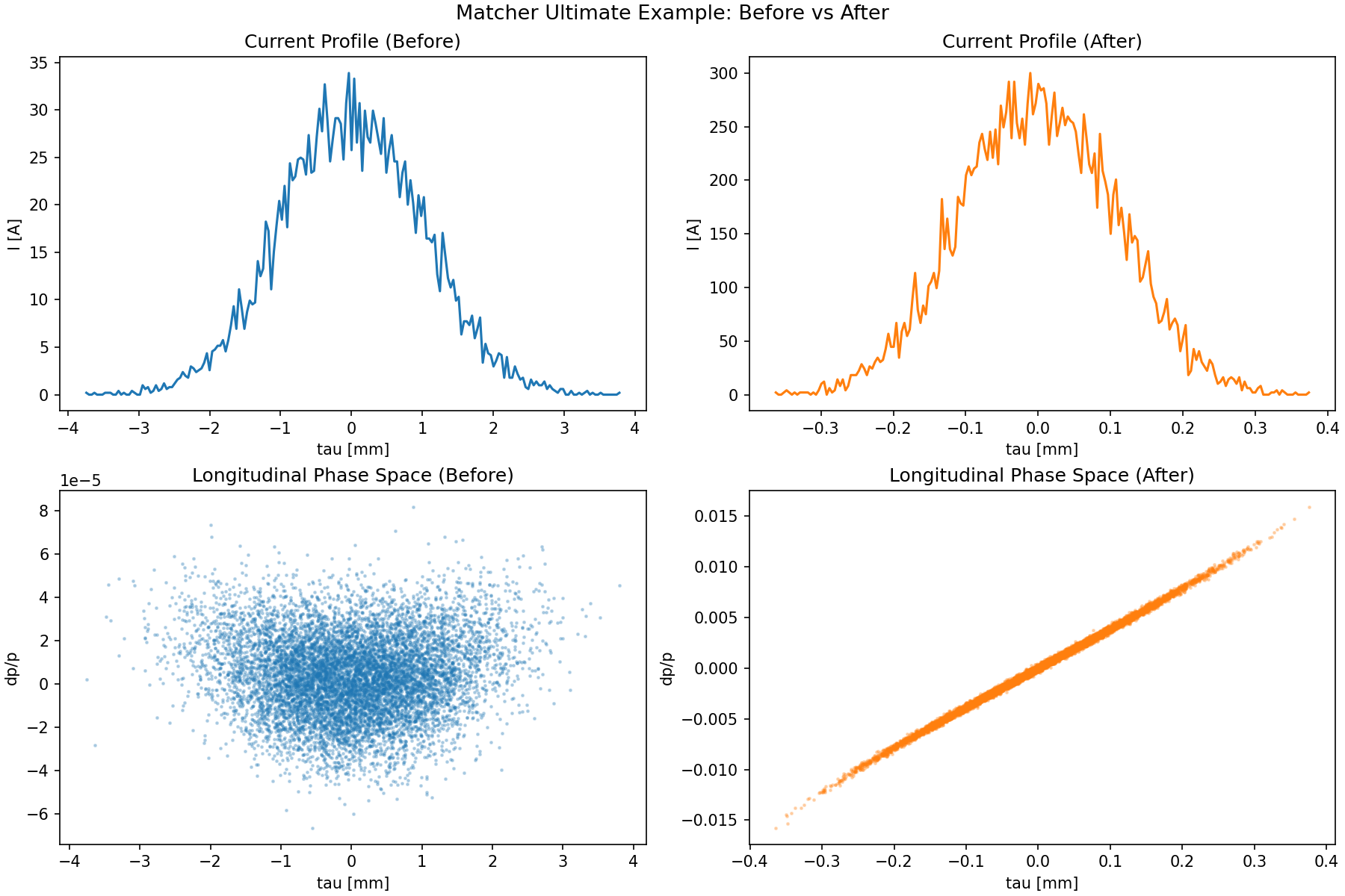
12) Ultimate Example: Custom Chicane Knob + Tracking Objective + Energy Target

Reference script:

• demos/ebeam/matcher_ex.py

This example combines three patterns in one workflow:

• Custom variable (Vary) with coupled lattice updates: one knob CHICANE_theta updates four dipole angles, edge angles (e1, e2), and chicane shoulder drifts consistently.
• Custom objective (Objective) with particle tracking inside residual evaluation: match a target peak current from tracked ParticleArray.
• Standard matcher target: final energy constraint with problem.target_twiss(end, "E", ...).

# Build a C-shape chicane section.
z_distance = 1.0
d_ref = Drift(l=0.5)
d12 = Drift(l=shoulders_from_theta(THETA0, z_distance))
d34 = Drift(l=shoulders_from_theta(THETA0, z_distance))

b1 = SBend(l=0.2, angle=-THETA0, e1=0.0, e2=-THETA0, tilt=0.0, fint=0.0, eid="B1")
b2 = SBend(l=0.2, angle=+THETA0, e1=THETA0, e2=0.0, tilt=0.0, fint=0.0, eid="B2")
b3 = SBend(l=0.2, angle=+THETA0, e1=0.0, e2=THETA0, tilt=0.0, fint=0.0, eid="B3")
b4 = SBend(l=0.2, angle=-THETA0, e1=-THETA0, e2=0.0, tilt=0.0, fint=0.0, eid="B4")
chicane = (b1, d12, b2, d_ref, b3, d34, b4)

# RF section and end marker.
c11 = Cavity(l=0.5, v=0.15, phi=0.0, freq=1.3e9, eid="C11")
c13 = Cavity(l=0.5, v=0.0166, phi=180.0, freq=3.9e9, eid="C13")
end = Marker(eid="END")

cell = [d_ref, c11, d_ref, c13, d_ref, *chicane, d_ref, end]
lat = MagneticLattice(cell)

tw0 = Twiss(beta_x=10.0, beta_y=10.0, emit_xn=1e-6, emit_yn=1e-6, E=0.005)
parray_init = generate_parray(tws=tw0, nparticles=10000, charge=250e-12,  chirp=0.0, sigma_p=SIGMA_P, sigma_tau=SIGMA_TAU_M)

# Track once before matching as a reference.
_tb, tracked_before = track(lat, copy.deepcopy(parray_init), print_progress=False)
i_before = peak_current(tracked_before)

# Create matcher problem.
problem = MatchProblem(lat, tw0)

# Custom composite variable: one theta knob drives the full chicane geometry.
def get_theta() -> float:
    return float(b2.angle)

def set_theta(theta: float) -> None:
    # 1) Update linked dipole angles.
    b1.angle = -theta
    b2.angle = +theta
    b3.angle = +theta
    b4.angle = -theta

    # 2) Update linked edge angles.
    b1.e1, b1.e2 = 0.0, -theta
    b2.e1, b2.e2 = +theta, 0.0
    b3.e1, b3.e2 = 0.0, +theta
    b4.e1, b4.e2 = -theta, 0.0

    # 3) Recompute chicane shoulder drifts from geometry.
    l_shoulder = shoulders_from_theta(theta, z_distance)
    d12.l = l_shoulder
    d34.l = l_shoulder

problem.add_variable(
    Vary(
        name="CHICANE_theta",
        getter=get_theta,
        setter=set_theta,
        limits=THETA_LIMITS,
    )
)

# Standard RF variables.
problem.vary_element(c11, quantity="v", limits=(0.10, 0.20), name="C11_v")
problem.vary_element(c11, quantity="phi", limits=(-40.0, 40.0), name="C11_phi")
problem.vary_element(c13, quantity="v", limits=(0.01, 0.025), name="C13_v")
problem.vary_element(c13, quantity="phi", limits=(90.0, 270.0), name="C13_phi")

# Custom tracking objective: peak current target.
class PeakCurrentObjective(Objective):
    """Tracking-based objective for peak current matching."""

    def __init__(self, parray_template, target_current: float, num_bins: int = 200, **kwargs):
        super().__init__(**kwargs)
        self.parray_template = parray_template
        self.target_current = float(target_current)
        self.num_bins = int(num_bins)

    def residuals(self, state):
        # Track a fresh copy each evaluation so residuals always use the same
        # initial particle distribution.
        parray = copy.deepcopy(self.parray_template)
        _tws_track, tracked = track(state.lat, parray, print_progress=False)
        i_peak = peak_current(tracked, num_bins=self.num_bins)
        return np.array([(i_peak - self.target_current) / self.target_current], dtype=float)

# Add custom objective to the problem.
problem.add_objective(
    PeakCurrentObjective(
        parray_template=parray_init,
        target_current=300,  # A
        name="peak_current_obj",
        weight=1e1,
    )
)

# Standard physics constraint: final energy at end marker (130 MeV).
problem.target_twiss(end, "E", value=0.13, weight=1e6)

# Solve.
result = problem.solve(solver="ls_trf", max_iter=MAX_ITER)

Run the full demo script:

python demos/ebeam/matcher_ex.py

Script output:

• console summary with optimized variables and achieved peak current
• generated figure: demos/ebeam/matcher_ex_before_after.png

Before/after image from the demo:

Regression + Benchmark Test

The test module unit_tests/ebeam_test/matcher/matcher_test.py includes:

• functional regression tests for matcher capabilities
• large-lattice optics cases
• benchmark timing test

Run full matcher tests:

pytest -q unit_tests/ebeam_test/matcher/matcher_test.py

Update benchmark baseline:

MATCHER_BENCH_UPDATE=1 pytest -q unit_tests/ebeam_test/matcher/matcher_test.py::test_match_optics_benchmark

Enforce speed regression guard (for example max 25% slowdown):

MATCHER_BENCH_ENFORCE=1 MATCHER_BENCH_MAX_SLOWDOWN=1.25 pytest -q unit_tests/ebeam_test/matcher/matcher_test.py::test_match_optics_benchmark