SpaceCharge Class

The SpaceCharge class models the space charge forces in a particle beam by solving the Poisson equation in the bunch frame. Then the Lorentz transformed electromagnetic field is applied as a kick in the laboratory frame. For the solution of the Poisson equation we use an integral representation of the electrostatic potential by convolution of the free-space Green's function with the charge distribution. The convolution equation is solved with the help of the Fast Fourier Transform (FFT). The same algorithm for solution of the 3D Poisson equation is used, for example, in ASTRA.

Parameters:

• step (int): Step size used in unit steps. Default is 1.
• nmesh_xyz (list): Defines the number of mesh points in each dimension for the 3D mesh. Default is [63, 63, 63].
• low_order_kick (bool): Whether to use a low-order approximation for the kick. Default is True.
• random_mesh (bool): If True, the mesh is shifted slightly at each step to reduce numerical noise. Default is False.
• random_seed (int): Seed for random number generation when random_mesh is True. Default is 10.

Methods:

__init__(self, step=1, **kwargs)

Constructor to initialize the SpaceCharge class with the specified parameters. It sets up the mesh, the randomization flag, and the random seed.

prepare(self, lat)

Prepares the simulation by checking the step size and setting the random seed if necessary.

sym_kernel(self, ijk2, hxyz)

Computes the symmetric kernel for the 3D Poisson equation solution using the convolution method. The kernel is used to calculate the electrostatic potential in the beam.

potential(self, q, steps)

Solves the Poisson equation for the electrostatic potential in the beam, given the charge distribution (q) and step sizes (steps). This method uses the Fast Fourier Transform (FFT) for efficient computation.

el_field(self, X, Q, gamma, nxyz)

Calculates the electric field in the rest frame of the bunch by using a 3D interpolation method. The result is Lorentz transformed to the laboratory frame.

apply(self, p_array, zstep)

Applies the space charge kick to the particle array (p_array) over a given path length (zstep). The method computes the electric field and updates the particle momenta according to the space charge forces.

__repr__(self) -> str

Returns a string representation of the SpaceCharge class, including key parameters like step size, mesh resolution, and randomization settings.

---

Summary

The SpaceCharge class simulates the space charge forces acting on a particle beam by solving the Poisson equation for the beam's charge distribution. The class computes the electric field using a convolution method and applies the resulting forces as kicks to the particle array. This model is crucial for understanding beam dynamics, especially in high-intensity beams where space charge effects are significant.

---

Space Charge Example

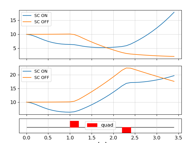
This example demonstrates how to simulate the impact of 3D space charge forces on the evolution of a particle beam through a simple FODO-like lattice. We compare tracking with and without space charge effects by plotting the resulting beta functions.

Step-by-Step

from ocelot import *
from ocelot.gui import *

# 1. Generate a test particle array with defined Twiss parameters
parray_init = generate_parray(
    nparticles=100000,
    tws=Twiss(beta_x=10, beta_y=10, E=0.01),  # E = 10 MeV
    sigma_tau=1e-4
)

# 2. Define a simple FODO-like lattice
qf = Quadrupole(l=0.2, k1=2)
qd = Quadrupole(l=0.2, k1=-2)
d = Drift(l=1)
m1 = Marker()  # Start of section
m2 = Marker()  # End of section

lat = MagneticLattice([m1, d, qf, d, qd, d, m2])

# 3. Tracking WITHOUT space charge
# Create navigator with step size 0.1 m
navi = Navigator(lat, unit_step=0.1)

# Add a dummy physics process to force tracking every step
emp = EmptyProc()
navi.add_physics_proc(emp, m1, m2)

parray = parray_init.copy()
tws_track_no_sc, _ = track(lat, parray, navi)

# 4. Tracking WITH 3D space charge
navi = Navigator(lat, unit_step=0.1)

# Create space charge process with default 3D mesh resolution
sc = SpaceCharge(nmesh_xyz=[63, 63, 63])
navi.add_physics_proc(sc, m1, m2)

parray = parray_init.copy()
tws_track_w_sc, _ = track(lat, parray, navi)

# 5. Plot beta functions with and without SC
fig, (ax_x, ax_y) = plot_API(lat, add_extra_subplot=True)

# Extract beta functions
s_no  = [tw.s for tw in tws_track_no_sc]
bx_no = [tw.beta_x for tw in tws_track_no_sc]
by_no = [tw.beta_y for tw in tws_track_no_sc]

s_sc  = [tw.s for tw in tws_track_w_sc]
bx_sc = [tw.beta_x for tw in tws_track_w_sc]
by_sc = [tw.beta_y for tw in tws_track_w_sc]

# Plot horizontal beta functions
ax_x.plot(s_no, bx_no, label="SC OFF")
ax_x.plot(s_sc, bx_sc, label="SC ON")
ax_x.set_ylabel(r"$\beta_x$ [m]")
ax_x.legend()

# Plot vertical beta functions
ax_y.plot(s_no, by_no, label="SC OFF")
ax_y.plot(s_sc, by_sc, label="SC ON")
ax_y.set_ylabel(r"$\beta_y$ [m]")
ax_y.set_xlabel("s [m]")
ax_y.legend()

plt.show()

Longitudinal Space Charge (LSC)

The LSC class simulates longitudinal space charge effects in particle beams. These effects arise due to the interaction of charged particles within a bunch, generating self-induced electric fields that distort the longitudinal phase space. This is particularly important for high-brightness or high-charge beams at low to moderate energies.

The space charge impedance is computed either for a smooth Gaussian-like distribution or using a stepped-profile approximation. The resulting wakefield is applied as a longitudinal kick to the beam during tracking.

---

Purpose

The LSC class models the 1D longitudinal space charge impedance and applies it to the beam using FFT-based wakefield computations. It allows users to choose between a smooth or stepped profile for the bunch and includes options for tuning the resolution of the impedance calculation.

---

Parameters

• step (int, default=1):
  Number of Navigator.unit_step segments between kicks. A step=1 means the wake is applied at each step.

• smooth_param (float, default=0.1):
  Defines the smoothing resolution of the longitudinal profile as
  resolution = std(p_array.tau()) * smooth_param.

• step_profile (bool, default=False):
  If True, uses a stepped profile approximation of the beam.
  If False, assumes a continuous longitudinal profile.

---

Methods

__init__(self, step=1, smooth_param=0.1, step_profile=False)

Initializes the LSC process with user-defined parameters.

apply(self, p_array, dz)

Applies the longitudinal space charge kick to a particle array over a longitudinal step dz.
Modifies particle momenta based on the calculated wakefield.

imp_lsc(self, gamma, sigma, w, dz)

Computes the longitudinal space charge impedance for a Gaussian-like distribution using beam energy gamma, transverse size sigma, frequency w, and step size dz.

imp_step_lsc(self, gamma, rb, w, dz)

Computes the impedance for a stepped beam profile. rb is the effective transverse beam radius.

wake2impedance(self, s, w)

Converts wakefield data w into impedance via a forward Fourier transform (exp(iwt)).

impedance2wake(self, f, y)

Performs an inverse Fourier transform (exp(-iwt)) to compute wakefield from impedance data.

wake_lsc(self, s, bunch, gamma, sigma, dz)

Computes the wakefield in real space for a given bunch distribution and beam parameters.

finalize(self, *args, **kwargs)

Finalizes the space charge computation at the end of tracking. Reserved for cleanup or optional output.

calculate_csr_wakes(self)

(Deprecated or internal use) Placeholder for compatibility with CSR-based wake computation.

plot_wake(self, p_array, lam_K1, itr_ra, s1, st)

Visualizes the longitudinal wake for diagnostic purposes. Intended for internal debugging or analysis.

---

Summary

The LSC class is part of the collective effects module in Ocelot. It provides a physics process that can be inserted into a beamline and used with the Navigator class to track particle beams under the influence of longitudinal space charge effects. The class offers flexibility in modeling beam profiles and efficiently computes impedance and wakefield using FFT methods.