This notebook was created by Sergey Tomin (sergey.tomin@desy.de). May 2025.

get_envelope Function Documentation

Overview

The get_envelope function computes statistical beam properties, commonly known as Twiss parameters and envelope characteristics, from a ParticleArray. This is essential for characterizing the beam's phase-space distribution.

info

As usual, Jupyter Notebook version can be found in Ocelot Repository

The function performs several key steps:

1. Particle Slicing (Optional): It can filter particles based on their longitudinal coordinate ($\tau$) to analyze a specific "slice" of the bunch.
2. Dispersion Correction (Optional): It can subtract the effects of linear dispersion from particle coordinates. Dispersion values can either be provided from a design Twiss object or automatically estimated from the particle data.
3. Coordinate Transformation: Ocelot's normalized transverse momenta ($\hat{x}' = p_x/p_0$, $\hat{y}' = p_y/p_0$) are converted to geometric angles ($x' = dx/ds$, $y' = dy/ds$) necessary for standard Twiss analysis.
4. Moment Calculation: It calculates first-order (centroids) and second-order moments (beam sizes, divergences, and correlations) of the particle distribution.
5. Twiss Parameter Derivation: Standard Twiss parameters ($\alpha, \beta$), geometric emittances, and normalized emittances are computed from these moments.

If, after optional slicing, fewer than three particles remain, the function returns a default (zeroed) Twiss object and logs a warning.

Syntax

def get_envelope(p_array, tws_i=None, bounds=None, slice=None, auto_disp=False):

Parameters

1. p_array (ParticleArray) The input particle array. The function uses the phase-space coordinates $x, \hat{x}', y, \hat{y}', \tau, p_{\text{ocelot}}$ for each particle, where:

   • $x, y$: transverse positions.
   • $\hat{x}' (= p_x/p_0), \hat{y}' (= p_y/p_0)$: Ocelot's normalized transverse momenta.
   • $\tau$: longitudinal coordinate.
   • $p_{\text{ocelot}} (= (E-E_0)/(p_0 c))$: Ocelot's relative energy deviation. For clarity in the formulas within this document, this quantity will be denoted as $\delta$. The code internally uses the variable p for this quantity.

2. tws_i (Twiss, optional) A reference Twiss object providing design dispersion values ($D_x, D'_x, D_y, D'_y$). Note $D'_x$ is the dispersive term for the angle $x'$. If provided, these values are used for dispersion correction. Default is None.

3. bounds (list, optional) A two-element list [left_bound, right_bound] defining a longitudinal slice for analysis, in units of $\sigma_\tau$ (the standard deviation of $\tau$ for the full beam).

   • If provided, particles are filtered to keep only those within the range: $$z_0 + \text{left\_bound} \cdot \sigma_{\tau} \le \tau_i \le z_0 + \text{right\_bound} \cdot \sigma_{\tau}$$ where $z_0$ is a reference longitudinal position determined by the slice parameter.
   • If None (default), all particles are used.

4. slice (str or None, optional) Determines the reference longitudinal position $z_0$ when bounds are active:

   • None (default): $z_0 = \langle \tau \rangle$ (the mean of $\tau$ for all particles).
   • "Imax": $z_0$ is set to the $\tau$ position where the beam current (longitudinal density) is maximal.

5. auto_disp (bool, optional) Controls automatic dispersion estimation:

   • If True AND tws_i is None, linear dispersion ($D_x, D'_x, D_y, D'_y$) is estimated directly from the statistical moments of the input p_array.
   • If False (default) or if tws_i is provided, no automatic estimation is performed.

Core Operations and Calculations

1. Particle Slicing (Filtering)

If bounds are specified, the particle data ($x, \hat{x}', y, \hat{y}', \tau, \delta$) is first filtered to include only particles within the defined longitudinal slice, as described under the bounds and slice parameters. (Recall $\delta$ is used here for Ocelot's relative energy deviation $p_{\text{ocelot}}$).

2. Dispersion Correction

Dispersion describes the coupling between particle energy deviation and transverse position/angle. This correction aims to analyze the "betatron" motion, which is the motion independent of energy effects.

• Source of Dispersion Values:

  • If tws_i is provided, its dispersion values ($D_x, D'_x, D_y, D'_y$) are used.
  • If tws_i is None and auto_disp is True, dispersion values are estimated from the particle distribution: $D_x = \frac{\langle (x-\bar{x})(\delta-\bar{\delta}) \rangle}{\langle (\delta-\bar{\delta})^2 \rangle}, \quad D'_x = \frac{\langle (\hat{x}'-\bar{\hat{x}'})(\delta-\bar{\delta}) \rangle}{\langle (\delta-\bar{\delta})^2 \rangle}$ and similarly for $D_y$ and $D'_y$. (Here, $\bar{x} = \langle x \rangle$, $\bar{\delta} = \langle \delta \rangle$, etc.)

• Applying the Correction: The particle coordinates are then corrected by subtracting the dispersive contribution. For each particle $i$:

  $$\begin{aligned} x_i &\leftarrow x_i - D_x \cdot \delta_i \\ \hat{x}'_i &\leftarrow \hat{x}'_i - D'_x \cdot \delta_i \\ y_i &\leftarrow y_i - D_y \cdot \delta_i \\ \hat{y}'_i &\leftarrow \hat{y}'_i - D'_y \cdot \delta_i \end{aligned}$$

  These dispersion-corrected coordinates are used for subsequent moment calculations.

3. Transformation to Geometric Angles

Twiss parameters are conventionally defined using geometric angles ($x' = dx/ds$). Ocelot stores normalized transverse momenta ($\hat{x}' = p_x/p_0$). A transformation is needed.

• Definitions and Key Relations:

  • Ocelot normalized transverse momentum: $\hat{x}' = p_x/p_0$.
  • Ocelot relative energy deviation (denoted as $\delta$ in this document): $\delta = \frac{\Delta E}{p_0 c} = \frac{E-E_0}{p_0c}$ where $E$ and $E_0$ are the total energies of the particle and reference particle, respectively, and $p_0$ is the total momentum of the reference particle.
  • Geometric angle: $x' = p_x/p_s$, where $p_s = \sqrt{p^2 - p_x^2 - p_y^2}$ is the longitudinal momentum of the particle, and $p$ is its total momentum.

• Relating Particle Total Momentum ($p$) to Reference Momentum ($p_0$) and $\delta$:

  The relativistic energy-momentum relation is $E^2 = (pc)^2 + (m_0c^2)^2$. For the reference particle: $E_0^2 = (p_0c)^2 + (m_0c^2)^2$. For an arbitrary particle: $E = E_0 + \delta p_0 c$. Substituting this into the particle's energy-momentum relation: $(pc)^2 = (E_0 + \delta p_0 c)^2 - (m_0c^2)^2 = E_0^2 + 2E_0 \delta p_0 c + (\delta p_0 c)^2 - (m_0c^2)^2$ Using $E_0^2 - (m_0c^2)^2 = (p_0c)^2$: $(pc)^2 = (p_0c)^2 + 2E_0 \delta p_0 c + (\delta p_0 c)^2$ Dividing by $(p_0c)^2$: $\left(\frac{p}{p_0}\right)^2 = 1 + \frac{2E_0 \delta}{p_0 c} + \delta^2$ Since $E_0/(p_0c) = 1/\beta_0$. Thus: $\left(\frac{p}{p_0}\right)^2 = 1 + \frac{2\delta}{\beta_0} + \delta^2$

• Exact Relation for Geometric Angle:

  Substituting $p_x = \hat{x}'p_0$, $p_y = \hat{y}'p_0$ and the expression for $(p/p_0)^2$ into $x' = p_x/\sqrt{p^2 - p_x^2 - p_y^2}$:

  $$x' = \frac{\hat{x}'}{\sqrt{\left(\frac{p}{p_0}\right)^2 - (\hat{x}'^2 + \hat{y}'^2)}} = \frac{\hat{x}'}{\sqrt{1 + \frac{2\delta}{\beta_0} + \delta^2 - (\hat{x}'^2 + \hat{y}'^2)}}$$

• Approximation Used in get_envelope:

  The square root term $(1+Z)^{-1/2}$ is approximated using the first-order Taylor expansion $1 - Z/2$. Let $Z = \frac{2\delta}{\beta_0} + \delta^2 - (\hat{x}'^2 + \hat{y}'^2)$. Then the correction factor is approximated as: $C \approx 1 - \frac{1}{2}Z = 1 - \frac{1}{2}\left(\frac{2\delta}{\beta_0} + \delta^2 - (\hat{x}'^2 + \hat{y}'^2)\right) = 1 - \frac{\delta}{\beta_0} - \frac{1}{2}\delta^2 + \frac{1}{2}(\hat{x}'^2 + \hat{y}'^2)$ The code further assumes an ultra-relativistic beam, where $\beta_0 \approx 1$. Thus, the implemented transformation (where $x'$ now denotes the geometric angle) becomes: $x' \approx \hat{x}' \left(1 - \delta - \frac{1}{2}\delta^2 + \frac{1}{2}\hat{x}'^2 + \frac{1}{2}\hat{y}'^2\right)$ And similarly for $y'$. The variables used in the code px, py, and p (Ocelot's $p_{\text{ocelot}}$) correspond to $\hat{x}'$, $\hat{y}'$, and $\delta$ respectively in this formula. This approximation effectively keeps terms up to second order in $\delta, \hat{x}', \hat{y}'$ within the multiplicative correction factor.

4. Calculation of Moments and Twiss Parameters

After the above corrections and transformations, the following are computed:

• Centroids (First-Order Moments):

  These are the mean values of the particle coordinates: $\langle x \rangle, \langle x' \rangle, \langle y \rangle, \langle y' \rangle, \langle \tau \rangle, \langle \delta \rangle$. Note: $\langle x' \rangle$ and $\langle y' \rangle$ are centroids of the geometric angles. $\langle \delta \rangle$ (mean relative energy deviation) is stored as tws.p.

• Covariances (Second-Order Moments):

  These are variances and covariances of the particle coordinates, taken with respect to their means (i.e., they are central moments). For example, the variance of $x$ is $\langle (x - \langle x \rangle)^2 \rangle$. The Twiss object stores them as:

  tws.xx = <(x - <x>)^2>
  tws.xpx = <(x - <x>)(x' - <x'>)>
  tws.pxpx = <(x' - <x'>)^2>
  // ... and similarly for y, y', τ, p_ocelot (δ), and cross-terms
  tws.yy = <(y - <y>)^2>
  tws.ypy = <(y - <y>)(y' - <y'>)>
  tws.pypy = <(y' - <y'>)^2>
  tws.tautau = <(τ - <τ>)^2>
  tws.pp = <(δ - <δ>)^2>
  // Cross-plane moments
  tws.xy = <(x - <x>)(y - <y>)>
  tws.xpy = <(x - <x>)(y' - <y'>)>
  tws.ypx = <(y - <y>)(x' - <x'>)>
  tws.pxpy = <(x' - <x'>)(y' - <y'>)>

• Emittances:

  • Geometric emittances (calculated from central moments): $\varepsilon_x = \sqrt{\langle (x - \langle x \rangle)^2 \rangle \langle (x' - \langle x' \rangle)^2 \rangle - \langle (x - \langle x \rangle)(x' - \langle x' \rangle) \rangle^2} = \sqrt{\text{tws.xx} \cdot \text{tws.pxpx} - \text{tws.xpx}^2}$ $\varepsilon_y = \sqrt{\langle (y - \langle y \rangle)^2 \rangle \langle (y' - \langle y' \rangle)^2 \rangle - \langle (y - \langle y \rangle)(y' - \langle y' \rangle) \rangle^2} = \sqrt{\text{tws.yy} \cdot \text{tws.pypy} - \text{tws.ypy}^2}$
  • Normalized emittances: $\varepsilon_{nx} = \beta_0 \gamma_0 \varepsilon_x, \quad \varepsilon_{ny} = \beta_0 \gamma_0 \varepsilon_y$ where $\beta_0, \gamma_0$ are relativistic factors of the reference particle (obtained from p_array.E).

• Twiss Parameters:

  $$\begin{aligned} \beta_x &= \frac{\text{tws.xx}}{\varepsilon_x}, &\quad \alpha_x &= -\frac{\text{tws.xpx}}{\varepsilon_x} \\ \beta_y &= \frac{\text{tws.yy}}{\varepsilon_y}, &\quad \alpha_y &= -\frac{\text{tws.ypy}}{\varepsilon_y} \end{aligned}$$

  The parameters $\gamma_x = (1+\alpha_x^2)/\beta_x$ and $\gamma_y = (1+\alpha_y^2)/\beta_y$ are calculated in Twiss class internally.

• Eigen-Emittances (eigemit_1, eigemit_2): These are calculated from the 4D transverse covariance matrix $\Sigma_{x,x',y,y'}$ to characterize beams with x-y coupling, representing the emittances in the decoupled eigenmodes.

Returns

Twiss

An instance of the Twiss class, populated with all the calculated centroids, moments, emittances, and Twiss parameters for the (optionally filtered and corrected) particle ensemble. Includes:

• E: Reference energy $E_0$.
• q: Total charge of the selected particles.
• p: Mean relative energy deviation $\langle \delta \rangle$ (corresponding to $\langle p_{\text{ocelot}} \rangle$).
• Centroids: x, px, y, py, tau. (px, py are centroids of geometric angles).
• Second-order moments: xx, xpx, pxpx, yy, ypy, pypy, tautau, pp, xy, xpy, ypx, pxpy.
• Emittances: emit_x, emit_y, emit_xn, emit_yn, eigemit_1, eigemit_2.
• Twiss functions: beta_x, alpha_x, beta_y, alpha_y.
• Dispersion (if calculated or passed): Dx, Dxp (as $D'_x$) , Dy, Dyp (as $D'_y$).

---

Examples of Use

The following examples illustrate how to use the get_envelope function directly and how its functionality is integrated within particle tracking simulations.

Simplest Example: Calculating Twiss from a ParticleArray

First, let's demonstrate the direct use of get_envelope. We will:

1. Define an initial set of Twiss parameters.
2. Generate a ParticleArray distribution matched to these Twiss parameters.
3. Use get_envelope to calculate the Twiss parameters back from the generated ParticleArray.

Ideally, the calculated Twiss parameters should closely match the initial ones.

NOTE: The output will show the Twiss parameters computed by get_envelope. Due to the statistical nature of particle generation and the finite number of particles, these will be very close but not exactly identical to tws0.

from ocelot import *
from ocelot.gui import *

# 1. Define arbitrary initial Twiss parameters
tws0 = Twiss(emit_xn=0.5e-6, emit_yn=0.5e-6, beta_x=10, beta_y=7, E=0.1)

# 2. Generate a ParticleArray matched to these Twiss parameters
# The generate_parray function aims to create a distribution whose statistical
# properties correspond to tws0. A chirp is added for later demonstration.
parray = generate_parray(tws=tws0, charge=250e-12, chirp=0.02)

# 3. Calculate Twiss parameters from the ParticleArray
# This is a direct call to get_envelope.
calculated_tws = get_envelope(parray)
print(calculated_tws)

    initializing ocelot...

    emit_x  = 2.5534086876131525e-09
    emit_y  = 2.547930016365793e-09
    emit_xn  = 4.996831723396634e-07
    emit_yn  = 4.986110369457615e-07
    beta_x  = 10.000263656786013
    beta_y  = 7.000081949297738
    alpha_x = 5.5915982949718466e-06
    alpha_y = 2.637941201691814e-05
    Dx      = 0.0
    Dy      = 0.0
    Dxp     = 0.0
    Dyp     = 0.0
    mux     = 0.0
    muy     = 0.0
    nu_x    = 0.0
    nu_y    = 0.0
    E       = 0.1
    s        = 0.0

Integration with track() function

The get_envelope function is automatically called within the track() function if calc_tws=True (which is the default). This allows for monitoring the beam envelope evolution along a beamline. Several arguments in track() are passed directly to get_envelope:

# Relevant arguments for get_envelope within track():
tws_track, parray_final = track(
         lattice,                      # MagneticLattice
         p_array_initial,              # ParticleArray
         navi=None,                    # Navigator
         calc_tws=True,                # If True (default), get_envelope() is called at each step.
         bounds=None,                  # Passed to get_envelope for slicing (width).
         slice=None,                   # Passed to get_envelope for slicing (position, e.g., "Imax").
         twiss_disp_correction=False   # Passed to get_envelope for dispersion correction.
 )

Let's create a simple lattice and track a beam through it, observing how get_envelope provides the evolving Twiss parameters.

Building a Sample Lattice

We will construct a lattice containing drifts, quadrupoles, and a four-bend chicane. Then, we'll calculate the design (ideal) Twiss parameters for this lattice based on our initial tws0.

d = Drift(l=1)
qf = Quadrupole(l=0.2, k1=1)
qd = Quadrupole(l=0.2, k1=-1)

# Chicane using rectangular dipoles
alpha_bend = 5 * np.pi / 180  # rad (corrected variable name)
b1 = Bend(l=0.2, angle=-alpha_bend, e2=-alpha_bend)
b2 = Bend(l=0.2, angle=alpha_bend, e1=alpha_bend)
b3 = Bend(l=0.2, angle=alpha_bend, e2=alpha_bend)
b4 = Bend(l=0.2, angle=-alpha_bend, e1=alpha_bend)

cell = [d, qf, d, qd, d, b1, d, b2, d, b3, d, b4, d, qf, d, qd, d]
lat = MagneticLattice(cell)

# Calculate design Twiss parameters for this lattice
tws_design = twiss(lat, tws0=tws0)

# Plot the design optical functions, including dispersion Dx
plot_opt_func(lat, tws_design, top_plot=["Dx"])
plt.show()

# The chicane will introduce longitudinal dispersion (R56)
_, R, _ = lat.transfer_maps(energy=tws0.E)
print(f"Calculated R56 of the lattice = {R[4, 5]*1e3:.4f} mm")

    Calculated R56 of the lattice = -17.6286 mm

The plot shows the design $\beta$-functions and, importantly, the horizontal dispersion $D_x$ generated by the chicane.

Tracking a ParticleArray: The Role of Dispersion Correction

Now, we will track the ParticleArray (generated earlier) through this lattice.

Scenario 1: Tracking without Dispersion Correction

By default, track() calls get_envelope without enabling its internal dispersion correction (unless twiss_disp_correction=True is set, or design dispersion is passed via tws_i to get_envelope). In regions with dispersion, the calculated transverse beam sizes and emittances will be inflated by the energy spread of the beam coupled through the dispersion function. This means the Twiss parameters calculated by get_envelope will reflect the projected phase space, not the purely betatronic motion.

parray1 = parray.copy() # Use a copy of the original particle array
tws_track_no_corr, _ = track(lat, p_array=parray1, calc_tws=True) # twiss_disp_correction defaults to False

# Plot the Twiss parameters calculated by get_envelope during tracking
plot_opt_func(lat, tws_track_no_corr, top_plot=["Dx"])
plt.show()

z = 10.6 / 10.6. Applied: .6. Applied:

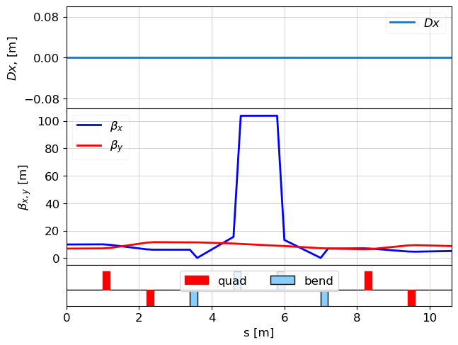
Observe in the resulting plot that $D_x$ (calculated from the particle statistics by get_envelope) is zero. This is because get_envelope (without auto_disp=True or tws_i) is not aware of the lattice dispersion. The calculated $\beta_x$ might also deviate significantly from the design tws_design.beta_x in dispersive regions, as the beam size includes the dispersive contribution $\sigma_x^2 = \epsilon_x \beta_x + (D_x \sigma_\delta)^2$.

Scenario 2: Tracking with Dispersion Correction Enabled

To obtain Twiss parameters that better reflect the betatronic motion and match the design optics (especially emittance and $\beta$-functions in dispersive regions), we need to enable dispersion correction within get_envelope. When using track(), this is done by setting twiss_disp_correction=True. This will make get_envelope automatically estimate and subtract the linear dispersion from the particle statistics (auto_disp=True behavior for get_envelope).

parray2 = parray.copy() # Use another copy
tws_track_with_corr, _ = track(lat, p_array=parray2, calc_tws=True, twiss_disp_correction=True)

# Plot the Twiss parameters calculated by get_envelope during tracking
plot_opt_func(lat, tws_track_with_corr, top_plot=["Dx"])
plt.show()

z = 10.6 / 10.6. Applied: .6. Applied:

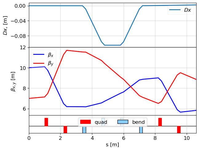
With twiss_disp_correction=True, the $D_x$ calculated by get_envelope from the particle statistics should now closely follow the design dispersion. The betatronic $\beta_x$ and emittance $\varepsilon_x$ will also be more representative of the intrinsic beam properties.

Observing Bunch Compression

Our lattice includes a chicane, which has an $R_{56}$ (longitudinal dispersion). If the incoming beam has an energy chirp (correlation between energy and longitudinal position), the chicane can compress or stretch the bunch. The parray was generated with a chirp. We can inspect the evolution of $\sigma_\tau$ (RMS bunch length), which is available from the tautau attribute of the Twiss objects returned by get_envelope at each step.

# Use tws_track_with_corr from the dispersion-corrected tracking
s_coords = np.array([tw.s for tw in tws_track_with_corr])
sigma_tau_values = np.array([np.sqrt(tw.tautau) for tw in tws_track_with_corr])

plt.figure() # Ensure a new figure for clarity
plt.plot(s_coords, sigma_tau_values * 1e3) # Convert sigma_tau to mm
plt.xlabel("s [m]")
plt.ylabel(r"RMS Bunch Length $\sigma_{\tau}$ [mm]")
plt.title("Bunch Length Evolution Through the Lattice")
plt.grid(True)
plt.show()

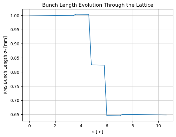
The plot of $\sigma_\tau$ vs. $s$ should show a change in bunch length as the beam passes through the chicane, demonstrating the effect of $R_{56}$ on a chirped beam. This highlights how get_envelope provides crucial second-order moments for analyzing various beam dynamics effects.