This notebook was created by Sergey Tomin (sergey.tomin@desy.de). January 2018.
5. Coherent Synchrotron Radiation (CSR)
Second-order tracking with CSR effects using 200,000 particles.
As an example, we simulate the BC2 bunch compressor of the European XFEL accelerator.
The CSR module in Ocelot uses a fast projected 1D model based on the approach from the CSRtrack code, following:
- Saldin et al, Radiative interaction of electrons in a bunch moving in an undulator, 1998,
- M. Dohlus, Two Methods for the Calculation of CSR Fields, 2003,
- M. Dohlus, T. Limberg, CSRtrack: FASTER CALCULATION OF 3-D CSR EFFECTS, 2004.
The particle tracking uses matrices up to the second order. CSR wake is calculated continuously through beam lines of arbitrary flat geometry. The transverse self-forces are neglected completely. The method calculates the longitudinal self-field of a one-dimensional beam that is obtained by a projection of the ‘real’ three-dimensional beam onto a reference trajectory. A smooth one-dimensional charge density is calculated by binning and filtering, which is crucial for the stability and accuracy of the simulation, since the instability is sensitive to high frequency components in the charge density.
This example covers:
- Initialization and placement of the
CSRclass - Second-order matrix-based tracking with CSR effects
- Use of the
Navigatorto assign physics processes - Lattice construction with
MagneticLattice
Requirements
-
in.fmt1: Initial beam distribution in CSRtrack format
(obtained from an s2e simulation performed with ASTRA + CSRtrack) -
out.fmt1: Output distribution after BC2 bunch compressor
(reference output from CSRtrack used for comparison)
import sys
sys.path.append("/Users/tomins/Nextcloud/DESY/repository/ocelot")
# the output of plotting commands is displayed inline within frontends,
# directly below the code cell that produced it
from time import time

# this python library provides generic shallow (copy) and deep copy (deepcopy) operations
from copy import deepcopy

# import from Ocelot main modules and functions
from ocelot import *

# import from Ocelot graphical modules
from ocelot.gui.accelerator import *
initializing ocelot...
Load beam distribution from CSRtrack format
# load and convert CSRtrack file to OCELOT beam distribution
# p_array_i = csrtrackBeam2particleArray("in.fmt1", orient="H")
# save ParticleArray to compresssed numpy array
# save_particle_array("test.npz", p_array_i)
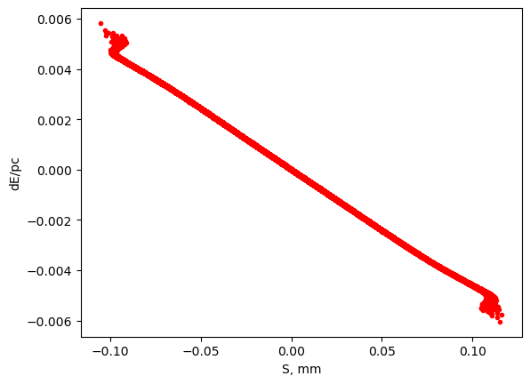
p_array_i = load_particle_array("csr_beam.npz")
# show the longitudinal phase space
plt.plot(-p_array_i.tau()*1000, p_array_i.p(), "r.")
plt.xlabel("S, mm")
plt.ylabel("dE/pc")
create BC2 lattice
b1 = Bend(l = 0.5001, angle=-0.0336, e1=0.0, e2=-0.0336, gap=0, tilt=0, eid='BB.393.B2')
b2 = Bend(l = 0.5001, angle=0.0336, e1=0.0336, e2=0.0, gap=0,  tilt=0, eid='BB.402.B2')
b3 = Bend(l = 0.5001, angle=0.0336, e1=0.0, e2=0.0336, gap=0, tilt=0,  eid='BB.404.B2')
b4 = Bend(l = 0.5001, angle=-0.0336, e1=-0.0336, e2=0.0, gap=0,  tilt=0, eid='BB.413.B2')

d_slope = Drift(l=8.5/np.cos(b2.angle))

start_csr = Marker()
stop_csr = Marker()

# define cell frome the bends and drifts
cell = [start_csr, Drift(l=0.1), b1 , d_slope  , b2, Drift(l=1.5),
        b3, d_slope, Marker(), b4, Drift(l= 1.), stop_csr]
Initialization tracking method and MagneticLattice object
# for second order tracking we have to choose SecondTM
method = {"global": SecondTM}

# for first order tracking uncomment next line
# method = {"global": TransferMap}

lat = MagneticLattice(cell, method=method)
Create CSR object
csr = CSR(n_bin=300, m_bin=5, sigma_min=.2e-6)
more details about CSR class can be found in Documentation.
Track particles with and without CSR effect
navi = Navigator(lat)

# track witout CSR effect
p_array_no = deepcopy(p_array_i)
print("\n tracking without CSR effect .... ")
start = time()
tws_no, p_array_no = track(lat, p_array_no, navi)
print("\n time exec:", time() - start, "sec")

# again create Navigator with needed step in [m]
navi = Navigator(lat)
navi.unit_step = 0.5 # m

# add csr process to navigator with start and stop elements
navi.add_physics_proc(csr, start_csr, lat.sequence[-1])

# tracking
start = time()
p_array_csr = deepcopy(p_array_i)
print("\n tracking with CSR effect .... ")
tws_csr, p_array_csr = track(lat, p_array_csr, navi)
print("\n time exec:", time() - start, "sec")
     tracking without CSR effect ....
    z = 21.610000676107052 / 21.610000676107052. Applied:
     time exec: 0.5144369602203369 sec

     tracking with CSR effect ....
    z = 21.610000676107052 / 21.610000676107052. Applied: CSR
     time exec: 13.474658012390137 sec
# recalculate reference particle
from ocelot.cpbd.beam import *
recalculate_ref_particle(p_array_csr)
recalculate_ref_particle(p_array_no)
# load and convert CSRtrack file to OCELOT beam distribution
# distribution after BC2
# p_array_out = csrtrackBeam2particleArray("out.fmt1", orient="H")
# save ParticleArray to compresssed numpy array
# save_particle_array("scr_track.npz", p_array_out)
p_array_out = load_particle_array("scr_track.npz")
# standard matplotlib functions
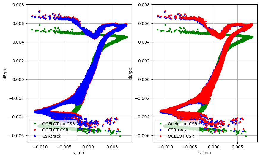
plt.figure(2, figsize=(10, 6))
plt.subplot(121)
plt.plot(p_array_no.tau()*1000, p_array_no.p(), 'g.', label="OCELOT no CSR")
plt.plot(p_array_csr.tau()*1000, p_array_csr.p(), 'r.', label="OCELOT CSR")
plt.plot(p_array_out.tau()*1000, p_array_out.p(), 'b.', label="CSRtrack")
plt.legend(loc=3)
plt.xlabel("s, mm")
plt.ylabel("dE/pc")
plt.grid(True)
plt.subplot(122)
plt.plot(p_array_no.tau()*1000, p_array_no.p(), 'g.', label="Ocelot no CSR")
plt.plot(p_array_out.tau()*1000, p_array_out.p(), 'b.', label="CSRtrack")
plt.plot(p_array_csr.tau()*1000, p_array_csr.p(), 'r.', label="OCELOT CSR")
plt.legend(loc=3)
plt.xlabel("s, mm")
plt.ylabel("dE/pc")
plt.grid(True)
plt.savefig("arcline_traj.png")
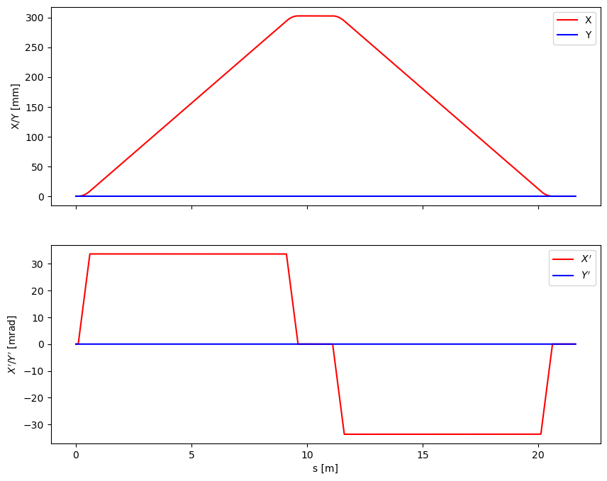
display trajectory of the reference particle in CSR region
fig = plt.figure(figsize=(10, 8))
ax1 = plt.subplot(211)
# ax1.plot(self.csr_traj[0, :], self.csr_traj[0, :] -self.csr_traj[3, :], "r", label="X")
ax1.plot(csr.csr_traj[0, :], csr.csr_traj[1, :] * 1000, "r", label="X")
ax1.plot(csr.csr_traj[0, :], csr.csr_traj[2, :] * 1000, "b", label="Y")
plt.legend()
plt.ylabel("X/Y [mm]")
plt.setp(ax1.get_xticklabels(), visible=False)
ax3 = plt.subplot(212, sharex=ax1)
ax3.plot(csr.csr_traj[0, :], csr.csr_traj[1 + 3, :] * 1000, "r", label=r"$X'$")
ax3.plot(csr.csr_traj[0, :], csr.csr_traj[2 + 3, :] * 1000, "b", label=r"$Y'$")
plt.legend()
plt.ylabel(r"$X'/Y'$ [mrad]")
plt.xlabel("s [m]")
plt.show()