This notebook was created by Sergey Tomin (sergey.tomin@desy.de). July 2019.

9. Accelerator-based THz source

This tutorial demonstrates coherent radiation from a macroparticle bunch using OCELOT's native Python SR module. For the introductory spontaneous-radiation examples, see PFS tutorial N1: Synchrotron radiation module (web version).

The physical model and its limitations for chirped THz bunches are discussed in G. Geloni, T. Tanikawa, and S. Tomin, Dynamical effects on superradiant THz emission from an undulator, Journal of Synchrotron Radiation 26 (2019), 737-749.

We first model a simplified accelerator and bunch-compression system. The undulator parameters are chosen to produce radiation in the THz range.

Accelerator
Coherent radiation from the beam

Accelerator

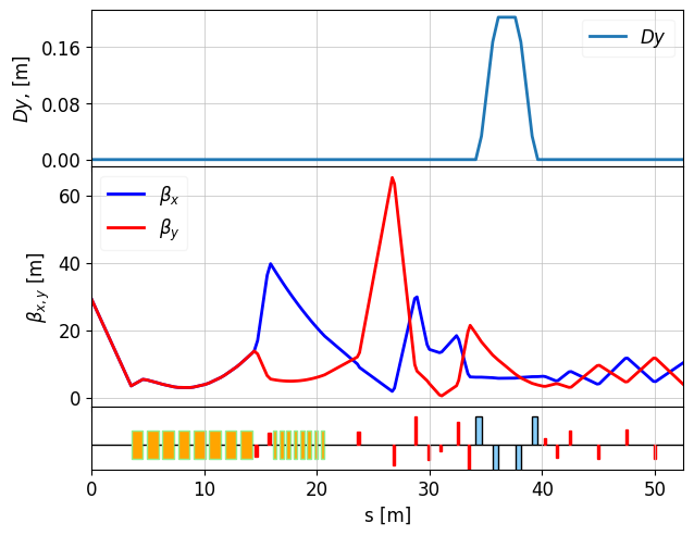
The accelerator contains a fundamental RF module, a third-harmonic linearizer, and a magnetic bunch compressor. It represents a simplified XFEL injector without the injector dogleg.

Lattice

# To activate interactive Matplotlib in the notebook
# %matplotlib notebook

from ocelot import * 
from ocelot.gui import *
import time

#Initial Twiss parameters
tws0 = Twiss()
tws0.beta_x = 29.171
tws0.beta_y = 29.171
tws0.alpha_x = 10.955
tws0.alpha_y = 10.955

tws0.E = 0.005

# Drifts
D0 = Drift(l=3.52)
D1 = Drift(l=0.3459)
D2 = Drift(l=0.2043)
D3 = Drift(l=0.85)
D4 = Drift(l=0.202)
D5 = Drift(l=0.262)
D6 = Drift(l=2.9)
D8 = Drift(l=1.8)
D9 = Drift(l=0.9)
D11 = Drift(l=1.31)
D12 = Drift(l=0.81)
D13 = Drift(l=0.50)
D14 = Drift(l=1.0)
D15 = Drift(l=1.5)
D18 = Drift(l=0.97)
D19 = Drift(l=2.3)
D20 = Drift(l=2.45)


# Quadrupoles
q1 = Quadrupole(l=0.3, k1=-1.537886, eid='Q1')
q2 = Quadrupole(l=0.3, k1=1.435078, eid='Q2')
q3 = Quadrupole(l=0.2, k1=1.637, eid='Q3')
q4 = Quadrupole(l=0.2, k1=-2.60970, eid='Q4')
q5 = Quadrupole(l=0.2, k1=3.4320, eid='Q5')
q6 = Quadrupole(l=0.2, k1=-1.9635, eid='Q6')
q7 = Quadrupole(l=0.2, k1=-0.7968, eid='Q7')
q8 = Quadrupole(l=0.2, k1=2.7285, eid='Q8')
q9 = Quadrupole(l=0.2, k1=-3.4773, eid='Q9')
q10 = Quadrupole(l=0.2, k1=0.780, eid='Q10')
q11 = Quadrupole(l=0.2, k1=-1.631, eid='Q11')
q12 = Quadrupole(l=0.2, k1=1.762, eid='Q12')
q13 = Quadrupole(l=0.2, k1=-1.8, eid='Q13')
q14 = Quadrupole(l=0.2, k1=1.8, eid='Q14')
q15 = Quadrupole(l=0.2, k1=-1.8, eid='Q15')


# SBends
b1 = SBend(l=0.501471120927, angle=0.1327297047, e2=0.132729705, tilt=1.570796327, eid='B1')
b2 = SBend(l=0.501471120927, angle=-0.1327297047, e1=-0.132729705, tilt=1.570796327, eid='B2')
b3 = SBend(l=0.501471120927, angle=-0.1327297047, e2=-0.132729705, tilt=1.570796327, eid='B3')
b4 = SBend(l=0.501471120927, angle=0.1327297047, e1=0.132729705, tilt=1.570796327, eid='B4')

# Cavities
c1 = Cavity(l=1.0377, v=0.01815975, freq=1300000000.0, eid='C1')
c3 = Cavity(l=0.346, v=0.0024999884, phi=180.0, freq=3900000000.0, eid='C3')


und = Undulator(lperiod=0.2, nperiods=20, Kx=30)
start_und = Marker()
end = Marker()
# Lattice 
cell = (D0, c1, D1, c1, D1, c1, D1, c1, D1, c1, D1, c1, D1, c1, D1, c1, D2, q1, D3,
        q2, D4, c3, D5, c3, D5, c3, D5, c3, D5, c3, D5, c3, D5, c3, D5, c3, D6, q3, D6,
        q4, D8, q5, D9, q6, D9, q7, D11, q8, D12, q9, D13, b1, D14, b2, D15, b3, D14, b4, D13,
        q10, D9, q11, D18, q12, D19, q13, D19, q14, D19, q15, D20, start_und, und, D14, end)

lat = MagneticLattice(cell, stop=start_und)

tws = twiss(lat, tws0)
plot_opt_func(lat, tws, legend=False, fig_name=100, top_plot=["Dy"])
plt.show()

png

The main longitudinal transport coefficients of the chicane can be calculated with chicane_RTU(yoke_len, dip_dist, r, type).

from ocelot.utils import *
R56, T566, U5666, Sref = chicane_RTU(yoke_len=0.5, dip_dist=D14.l * np.cos(b1.angle), r=b1.l/b1.angle, type="c")
print("bunch compressor R56 = ", R56, " m")

bunch compressor R56 =  -0.04751528087514777  m

Simple compression scenario

We consider here a basic compression scheme consisting of an accelerating module, a third-harmonic linearizer, and a magnetic chicane. For a comprehensive overview of bunch-compression physics, the following references are highly recommended:

Linear Compression with a Chicane

To compress a bunch longitudinally, the tail must have a shorter time of flight through some beamline section than the head. A standard technique is first to introduce a correlation between a particle’s longitudinal position and its energy using RF acceleration.

At the exit of a linac that induces a linear energy chirp

\delta' = \frac{1}{E_0}\frac{dE}{ds},

the mapping of the longitudinal coordinate $s$ and the relative energy deviation $\delta$ is

\begin{aligned} s_1 &= s_0,\\ \delta_1 &= \delta' s_0 + \delta_{i}, \end{aligned}

where $\delta_i = \Delta E_i / E_0$ denotes the uncorrelated energy spread.

Passing this beam through a magnetic chicane with longitudinal dispersion $R_{56}$ , the transformation (to first order) becomes

\begin{aligned} s_2 &= s_1 - R_{56}\,\delta_1 = (1 - \delta' R_{56})\, s_0 + R_{56}\,\delta_i,\\[2pt] \delta_2 &= \delta_1. \end{aligned}

Assuming $\langle s_0 \delta_i \rangle = 0$ , the rms bunch length after the chicane is

\sigma_{s_2} = \sqrt{ (1 - \delta' R_{56})^2\, \sigma_{s_0}^2 + R_{56}^2 \sigma_{\delta_i}^2 }.

The compression factor is

C = \frac{\sigma_{s_0}}{\sigma_{s_2}}.

Assuming negligible uncorrelated energy spread and choosing
$\delta' = -10$ and $R_{56} = -0.048~\mathrm{m}$ , the compression factor becomes

C = \frac{1}{1 - \delta' R_{56}} = 1.9.

Linearization with a Third-Harmonic RF System

Nonlinearities from the RF fields and from the magnetic chicane introduce curvature in the longitudinal phase space, degrading compression.
A higher-harmonic RF module can be used to compensate these nonlinearities and linearize the phase space. For the fundamental RF and its $n$ -th harmonic (with $n=3$ at the European XFEL), the normalized RF amplitudes must satisfy

\begin{bmatrix} 1 & 0 & 1 & 0 \\ 0 & -k & 0 & -n k \\ -k^2 & 0 & -(nk)^2 & 0 \\ 0 & k^3 & 0 & (nk)^3 \end{bmatrix} \begin{bmatrix} V_1 \cos\phi_1 \\ V_1 \sin\phi_1 \\ V_{13} \cos\phi_{13} \\ V_{13} \sin\phi_{13} \end{bmatrix} = \frac{1}{e} \begin{bmatrix} E_1 - E_0 \\ E_1\delta_2' - E_0\delta_0' \\ E_1\delta_2'' - E_0\delta_0'' \\ E_1\delta_2''' - E_0\delta_0''' \end{bmatrix}.

We assume initial conditions:

E_0 = 5~\mathrm{MeV}, \qquad \delta_0' = \delta_0'' = \delta_0''' = 0.

As a target after the RF system (and before the chicane), we choose:

E_1 = 130~\mathrm{MeV}, \qquad \delta_2' = -10, \qquad \delta_2'' = \delta_2''' = 0.

Thus, the right-hand side becomes

\begin{bmatrix} 125 \\ -1300 \\ 0 \\ 0 \end{bmatrix}.

Additional Contribution from the Undulator

Note:
The earlier estimate of $R_{56}$ included only the chicane.
The undulator also contributes to longitudinal dispersion.

For an undulator with large $K$ -value, the longitudinal dispersion is

R_{56} = -\frac{L_u}{\gamma^2}\left( 1 + \frac{K^2}{2} \right) \approx -0.028~\mathrm{m}.

Including this contribution, the total compression factor becomes

C = \frac{1}{1 - \delta' R_{56}} = 4.1.

import scipy.optimize

# M*a = b
k = 2*np.pi/3e8*1.3e9
n = 3 
M = np.array([[1,     0,      1,          0],
             [0,      -k,     0,       -(n*k)],
             [-k**2,  0,   -(n*k)**2,     0],
             [0,      k**3,   0,      (n*k)**3]])


b = np.array([125, -1300, 0, 0])
def F(x):
    V1 = x[0]
    phi1 = x[1]
    V13 = x[2]
    phi3 = x[3]
    V = np.array([V1*np.cos(phi1*np.pi/180),
             V1*np.sin(phi1*np.pi/180),
             V13*np.cos(phi3*np.pi/180),
             V13*np.sin(phi3*np.pi/180)]).T
    return np.dot(M, V) - b

x = scipy.optimize.broyden1(F, [150, 10, 20, 190])
V1, phi1, V13, phi13 = x
print("V1 = ", V1, " MeV")
print("phi1 = ", phi1)
print("V13 = ", V13, " MeV")
print("phi13 = ", phi13)

V1 =  150.53461559069942  MeV
phi1 =  20.905449652203075
V13 =  15.751142631398178  MeV
phi13 =  187.25608275724716

Update the cavity parameters in the lattice.

# Set the new parameters
# NOTE: OCELOT cavity voltage is in GeV, so convert the calculated voltage from MeV by a factor of 1/1000
# The main RF module and the linearizer each contain eight cavities
c1.v = V1/8/1000
c1.phi = phi1
c3.v = V13/8/1000
c3.phi = phi13

# Update the lattice
lat.update_transfer_maps()

Generate the electron beam

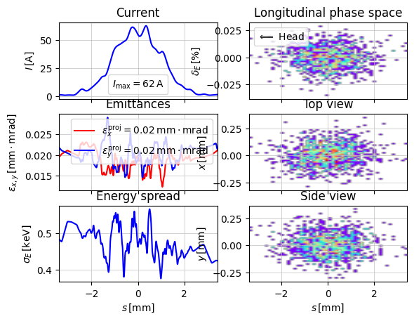
For accurate coherent-radiation results, use at least several tens of thousands of macroparticles. This shortened example uses 1000 particles to keep the runtime manageable.

np.random.seed(30)
parray = generate_parray(sigma_x=0.0001, sigma_px=2e-05, sigma_y=None, sigma_py=None, 
                         sigma_tau=0.001, sigma_p=0.0001, chirp=0.0, charge=0.5e-09, 
                         nparticles=1000, energy=0.005, tau_trunc=None, shape="gauss")

show_e_beam(parray,nparts_in_slice=50,smooth_param=0.1, nbins_x=50, nbins_y=50, nfig=10)
plt.show()

png

Track to the undulator entrance

navi = Navigator(lat)
tws_track, parray = track(lat, parray, navi)
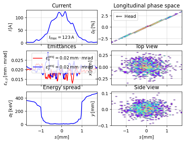
show_e_beam(parray, nparts_in_slice=50,smooth_param=0.1, nbins_x=50, nbins_y=50, nfig=201)
plt.show()

png

parray.E

np.float64(0.1300000026775309)

Coherent radiation from the beam

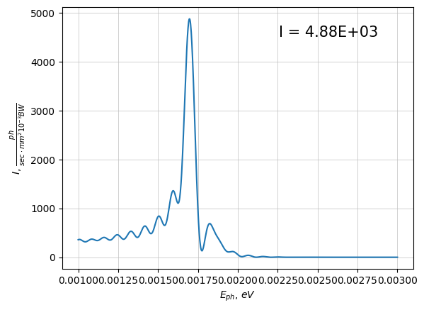
coherent_radiation tracks every macroparticle through the selected lattice and sums the complex radiation fields before calculating intensity. The stored photon distributions are normalized per bunch, per square millimetre, and per $10^{-3}$ relative bandwidth. No repetition rate is applied; multiply by the bunch repetition rate in hertz to obtain photons per second.

from ocelot.rad import *
lat = MagneticLattice(cell, start=start_und, stop=end)

screen = Screen()
screen.z = 1000.0
screen.size_x = 15
screen.size_y = 15
screen.nx = 1
screen.ny = 1
screen.start_energy = 0.001  # eV
screen.end_energy = 3e-3  # eV
screen.num_energy = 1001

# to estimate radiation properties we need to create beam class 

beam = Beam()
beam.E = 0.13

# NOTE: this function estimates spontaneous emission only
print_rad_props(beam, K=und.Kx, lu=und.lperiod, L=und.l, distance=screen.z)

********* ph beam ***********
Ebeam        :  0.13  GeV
K            :  30
B            :  1.6065  T
lambda       :  6.96835E-04  m
Eph          :  1.77925E-03  eV
1/gamma      :  3930.7605  um
sigma_r      :  5941.5531  um
sigma_r'     :  9332.9698  urad
Sigma_x      :  5941.5531  um
Sigma_y      :  5941.5531  um
Sigma_x'     :  9332.9698 urad
Sigma_y'     :  9332.9698 urad
H. spot size :  9332.9717 / 9.333  mm/mrad
V. spot size :  9332.9717 / 9.333  mm/mrad
I            :  0.0  A
Nperiods     :  20.0
distance     :  1000.0  m
flux tot     :  0.00E+00  ph/sec/0.1%BW
flux density :  0.00E+00  ph/sec/mrad^2/0.1%BW;    0.00E+00  ph/sec/mm^2/0.1%BW
brilliance   :  0.00E+00  ph/sec/mrad^2/mm^2/0.1%BW

start = time.time()
screen_i = coherent_radiation(lat, screen, parray, accuracy=1)
print()
print("time exec: ", time.time() - start, " s")
show_flux(screen_i, unit="mm", title="")

png

Beam after the undulator

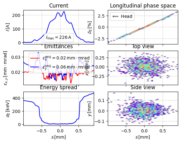
The bunch is compressed by approximately a factor of two while traversing the undulator. This is consistent with the estimate in the simple compression scenario, where the undulator's longitudinal dispersion is included.

show_e_beam(parray, nparts_in_slice=50,smooth_param=0.1, nbins_x=50, nbins_y=50,  nfig=203)
plt.show()

png

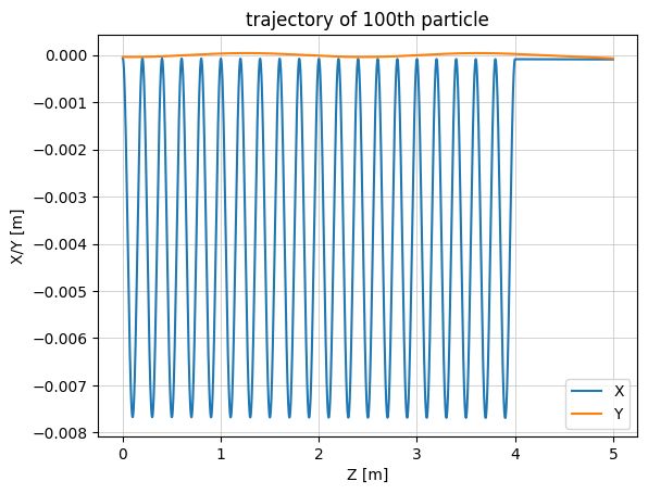
Electron trajectories

It is often useful to inspect the particle trajectories used in the radiation calculation. After the calculation, a BeamTraject object is attached to the Screen:

screen.beam_traj = BeamTraject()

Specify the macroparticle index to retrieve a trajectory, for example:

x = screen.beam_traj.x(n=0)

n = 100
x = screen.beam_traj.x(n)
y = screen.beam_traj.y(n)
z = screen.beam_traj.z(n)
plt.title("trajectory of " + str(n)+"th particle")
plt.plot(z, x, label="X")
plt.plot(z, y, label="Y")
plt.xlabel("Z [m]")
plt.ylabel("X/Y [m]")
plt.legend()
plt.show()

png

Contents​

Accelerator​

Lattice​

Simple compression scenario​

Linear Compression with a Chicane​

Linearization with a Third-Harmonic RF System​

Additional Contribution from the Undulator​

Generate the electron beam​

Track to the undulator entrance​

Coherent radiation from the beam​

Beam after the undulator​

Electron trajectories​

Contents